AI 学习笔记
 AI学习笔记。
AI 学习笔记
机器学习简介
Different types of Functions
Regression : The function outputs a scalar(标量).
- predict the PM2.5
Classification : Given options (classes), the function outputs the correct one.
- Spam filtering
Structured Learning : create something with structure(image, document)
Example : YouTube Channel
1.Function with Unknown Parameters.
2.Define Loss from Training Data
- Loss is a function of parameters
- Loss : how good a set of values is.
- L is mean absolute error (MAE)
- L is mean square error (MSE)
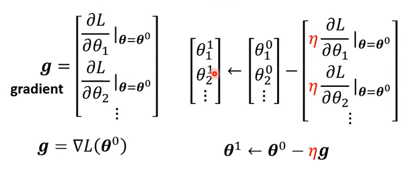
3.Optimization
Gradient Descent
- (Randomly) Pick an initial value :
- Compute :
Negative : Increase w
Positive : Decrease w
η:learning rate (hyperparameters)
- Update w iteratively
- Local minima
- global minima
类似一个参数,推广到多个参数。
Linear Models
Linear models have severe limitation. Model Bias.
We need a more flexible model!
curve = constant + sum of a set of Hard Sigmoid Function
线性代数角度:
Loss
- Loss is a function of parameters L(θ)
- Loss means how good a set of values is.
Optimization of New Model
- (Randomly) Pick initial values θ^0
1 epoch = see all the batched once
update : update θ for each batch
Sigmoid -> ReLU (Rectified Linear Unit)
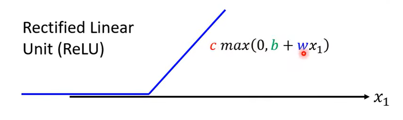
统称为 Activation function
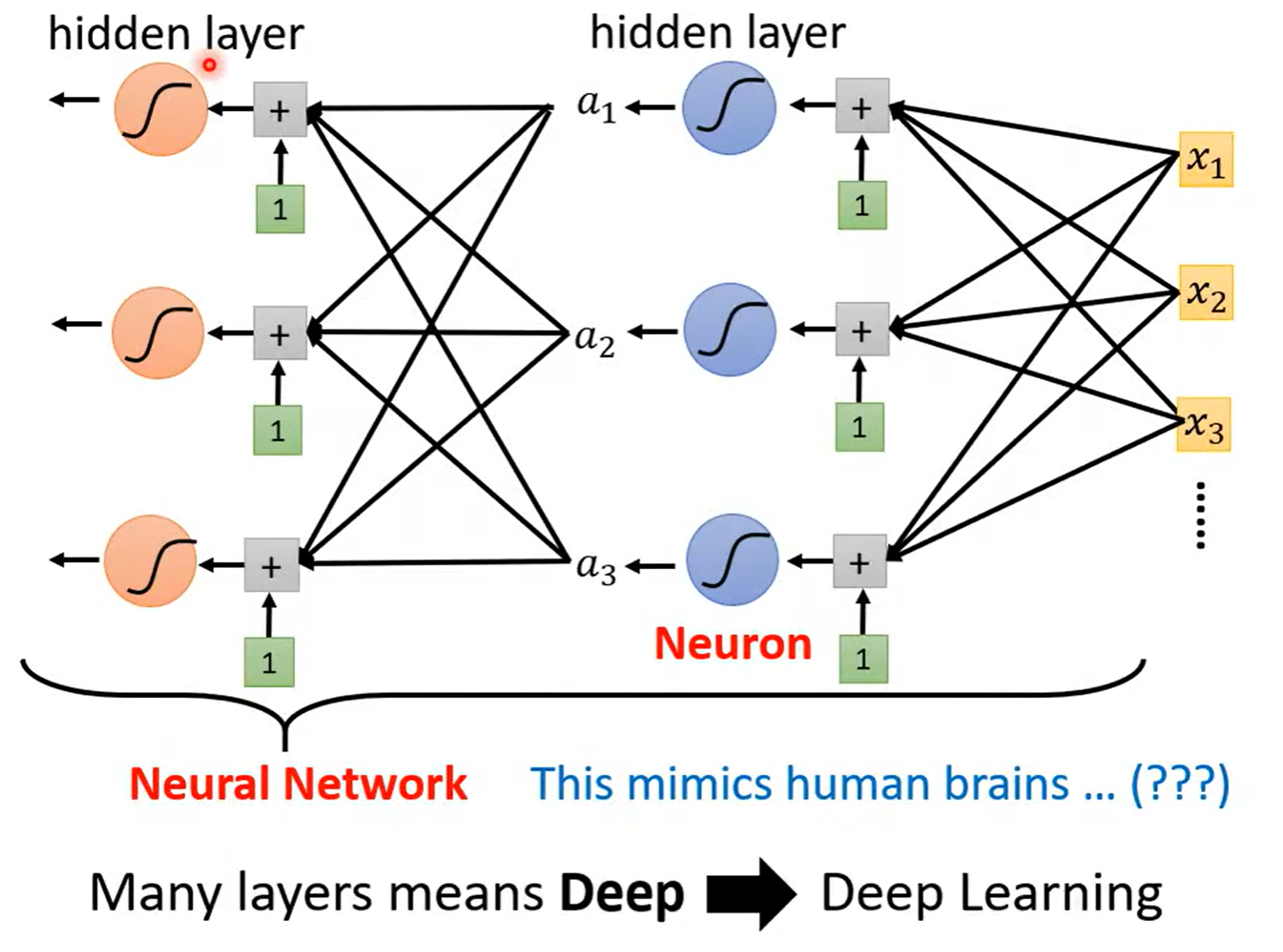
Neural Network
PyTorch
Python3中机器学习框架
dataset = MyDataset(file)
dataloader = DataLoader(dataset, batch_size = size , shuffle = True)
Training : True
Testing : False
from torch.utils.data import Dataset, DateLoader
class MyDataset(Dataset):
	def __init__(self, file): # read data & preprocess
		self.data = ...
	def __getitem__(self,index): #return one sample at a time
		return self.data[index]
	def __len__(self): #return the size of the dataset
		return len(self.data)
Tersors
High-dimensional matrices(arrays)
.shape() # show the dimension
#Directly from data (list or numpy.ndarray)
x = torch.tensor([1, -1], [-1, 1])
x = torch.from_numpy(np.array([[1, -1], [-1, 1]]))
#Tensor of constant zeros & ones
x = torch.zeros([2, 2])
x = torch.ones([1, 2, 5])
x+y x-y y=x.pow(2) y=x.sum() y=x.mean()
#Transpose : transpose two specified dimensions
x = x.transpose(dim0,dim1) # change the dimension dim0 and dim1
#Squeeze : remove the specified dimension with length 1
x = x.squeeze(1)
#unsqueeze expand a new dimension
x = x.unsqueeze(1)
PyTorch
dataset = MyDataset(file)
dataloader = Dataloader(dataset, batch_size, shuffle = True)
shuffle : Training -> true
		  Testing -> false
Tersors
- High-dimensional matrices(matrix used in mathematics, arrays)
dim in PyTorch == axis in NumPy
dimensional
Check with.shape()
Creating Tensors
-
Directly from data (list or numpy.ndarray)
x = torch.tensor([1, -1], [-1, 1]) x = torch.from_numpy(np.array([[1, -1], [-1, 1]])) -
Tensor of constant zeros & ones
x = torch.zeros([2,2])
x = torch.ones([1, 2, 5])
- Common Operations
addition subtraction power summation mean
- transpose
x.shape
x.transpose(0,1)
Unsqueeze : expand a new dimension
x = x.unsqueeze(1)
**Cat **: conncatenate multiple tensors 合并多个矩阵
torch.cat([x, y, z], dim = 1)
Data Type: Using different data types for model and data will case errors.
32-bit -torch.float
64-bit -torch.long
Device
- Tensors & modules will be computed with CPU by default
- Use .to() to move tensors to appropriate devices
- CPU
x = x.to('cpu') - ```py x = x.to('cuda')
- CPU
- GPU
- check if your computer has NVIDIA GPU
torch.cuda.is_available() - Multiple GPUs : specify- ``` 'cuda:0', 'cuda:1', 'cuda:2',...
- check if your computer has NVIDIA GPU
Cradient Calculation
import torch
# 定义一个需要求导的张量 x,并将 requires_grad 参数设置为 True
x = torch.tensor([[1., 0.], [-1., 1.]], requires_grad=True)
# 计算 x 的平方并对其进行求和,得到张量 z
z = x.pow(2).sum()
# 对张量 z 进行反向传播,自动计算出 x 的梯度
z.backward()
# 输出 x 的梯度
print(x.grad)
torch.nn
Network Layers
- Linear Layer (Fully-connected Layer)
nn.linear(in_features, out_features) #### Non-linear Activation Functions```pynn.Sigmoid()nn.ReLU()
Build your own neural network
import torch.nn as nn
class MyModel(nn.Module):
    #initialize your model & define layers
	def __init__(self):
		super(MyModel, self).__init__()
		self.net = nn.Sequential(
			nn.Linear(10, 32),
			nn.Sigmoid(),
			nn.Linear(32,1)
		)
	#compute output of your nn
	def forward(self, x):
		return self.next()
Loss Functions
- Mean squared Error (for regression tasks)
criterion = nn.MSELoss()
- Cross Entropy (for classification tasks) 交叉熵
criterion = nn.CrossEntropyLoss()
loss = criterion(model_output, expected_value) ### torch.optim- Stochastic Gradient Descent (SGD) - ```py torch.optim.SGD(model.parameters(), lr, momentum = 0)- For every batch of data
- Call optimizer.zero_grad() to reset gradients of model parameters.
- Call loss.backward() to backpropagate gradients of prediction loss
- Call optimizer.step() to adjust model parameters
Neural Network Training Setup
dataset = MyDataSet(file)
tr_set = DataLoader(dataset, 16, shuffle = True)
model = MyModel().to(device)
criterion = nn.MSELoss()
optimizer = torch.optim.SGD(model.parameters(), 0.1)
Training Loop
for epoch in range(n_epochs):  # Iterate over n_epochs
    model.train()  # Set the model to training mode
    for x, y in tr_set:  # Iterate over the training set
        optimizer.zero_grad()  # Clear the gradients
        x, y = x.to(device), y.to(device)  # Move data to the device (e.g., GPU)
        pred = model(x)  # Forward pass, compute predictions
        loss = criterion(pred, y)  # Compute the loss
        loss.backward()  # Backward pass, compute gradients
        optimizer.step()  # Update the model's parameters using the gradients
Validation Loop
model.eval()  # Set the model to evaluation mode
total_loss = 0

for x, y in dv_set:  # Iterate over the validation set
    x, y = x.to(device), y.to(device)  # Move data to the device
    with torch.no_grad():  # Disable gradient computation
        pred = model(x)  # Forward pass, compute predictions
        loss = criterion(pred, y)  # Compute the loss
    total_loss += loss.cpu().item() * len(x)  # Accumulate the loss
avg_loss = total_loss / len(dv_set)  # Calculate the average loss per sample
Testing Loop
model.eval()  # Set the model to evaluation mode
preds = []

for x in tt_set:  # Iterate over the test set
    x = x.to(device)  # Move data to the device
    with torch.no_grad():  # Disable gradient computation
        pred = model(x)  # Forward pass, compute predictions
        preds.append(pred.cpu())  # Append the predictions to the list
Data, demo1
Load data :
use pandas to load a csv file
train_data = pd.read_cav('./name.csv').drop(columns=['date']).values
x_train, y_train = train_data[:,:-1], train_data[:,:-1]
Dataset
init : Read data and preproces
getitem : Return one sample at a time, In this case, one sample includes a 117 dimensional feature and a label
len : Return the size of the dataset. In this case, it is 2699
class COVID19Dataset(Dataset):
    '''
    x: np.ndarray  特征矩阵.
    y: np.ndarray  目标标签, 如果为None,则是预测的数据集
    '''
    def __init__(self, x, y=None):
        if y is None:
            self.y = y
        else:
            self.y = torch.FloatTensor(y)
        self.x = torch.FloatTensor(x)

    def __getitem__(self, idx):
        if self.y is None:
            return self.x[idx]
        return self.x[idx], self.y[idx]

    def __len__(self):
        return len(self.x)
Dataloader
train_loader = DataLoader(train_dataset, batch_size = 32, shuffle = True, pin_memory = True)
Model
class My_Model(nn.Module):
    def __init__(self, input_dim):
        super(My_Model, self).__init__()
        # TODO: 修改模型结构, 注意矩阵的维度(dimensions)
        self.layers = nn.Sequential(
            nn.Linear(input_dim, 16),
            nn.ReLU(),
            nn.Linear(16, 8),
            nn.ReLU(),
            nn.Linear(8, 1)
        )

    def forward(self, x):
        x = self.layers(x)
        x = x.squeeze(1) # (B, 1) -> (B)
        return x
Criterion
criterion = torch.nn.MSELoss(reduction = 'mean')
Optimizer
optimizer = torch.optim.SGD(model.parameters(), lr = 1e-5, momentum = 0.9)
Training Loop
Documentation and Common Errors
read pytorch tutorial
Colab(highly recommended)
Officially begin
Deep = Many hidden layers
Neurall Network
Find a function in function set.
Goodness of function
Pick the best function
Backpropagation - Backward Pass(反向传播)
反向的neural network
Regression
- Stock Market Forecast
- Self-driving Car
- Recommendation
Step 1 : Model
A set of function
Step 2 : Goodness of Function
Loss function L:
Step 3 :Best Function
In linear regression, the loss function L is convex.
Overfitting
Regularization
不需要考虑bias,调整平滑程度,smooth
- Gradient descent
- Overfitting and Regularization
Classification
Training data for Classification
pair
Ideal Alternatives
Function(Model):
lossfunction:
The number of times of get incotrrect results on training data.
Find the best function;
- Example : Perceptron, SVM
Prior
Gaussian
Maximum Likelihood
2D array or 3D array mean the array with 2 or 3 axes respectively, but the n-dimensional vector mean the vector of length n.
Learn something that can really differ you from others.

 浙公网安备 33010602011771号