Python for Data Science - Extreme value analysis using univariate methods

Chapter 5 - Outlier Analysis

Segment 8 - Extreme value analysis using univariate methods

import numpy as np
import pandas as pd

import matplotlib.pyplot as plt
from pylab import rcParams

%matplotlib inline
rcParams['figure.figsize'] = 5,4

address = '~/Data/iris.data.csv'
df = pd.read_csv(filepath_or_buffer=address, header=None, sep=',')

df.columns=['Sepal Length','Sepal Width','Petal Length','Petal Width', 'Species']

X = df.iloc[:,0:4].values
y = df.iloc[:,4].values
df[:5]

	Sepal Length	Sepal Width	Petal Length	Petal Width	Species
0	5.1	3.5	1.4	0.2	setosa
1	4.9	3.0	1.4	0.2	setosa
2	4.7	3.2	1.3	0.2	setosa
3	4.6	3.1	1.5	0.2	setosa
4	5.0	3.6	1.4	0.2	setosa

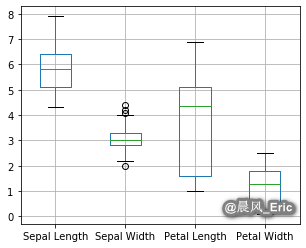
Identifying outliers from Tukey boxplots

df.boxplot(return_type='dict')
plt.plot()

[]

Sepal_Width = X[:,1]
iris_outliers = (Sepal_Width > 4)
df[iris_outliers]

	Sepal Length	Sepal Width	Petal Length	Petal Width	Species
15	5.7	4.4	1.5	0.4	setosa
32	5.2	4.1	1.5	0.1	setosa
33	5.5	4.2	1.4	0.2	setosa

Sepal_Width = X[:,1]
iris_outliers = (Sepal_Width < 2.05)
df[iris_outliers]

	Sepal Length	Sepal Width	Petal Length	Petal Width	Species
60	5.0	2.0	3.5	1.0	versicolor

Applying Tukey outlier labeling

pd.options.display.float_format = '{:.1f}'.format
X_df = pd.DataFrame(X)
print(X_df.describe())

0 1 2 3
count 150.0 150.0 150.0 150.0
mean 5.8 3.1 3.8 1.2
std 0.8 0.4 1.8 0.8
min 4.3 2.0 1.0 0.1
25% 5.1 2.8 1.6 0.3
50% 5.8 3.0 4.3 1.3
75% 6.4 3.3 5.1 1.8
max 7.9 4.4 6.9 2.5