实验5 支持向量机分类实验

作者：康慎吾

一、实验要求
在计算机上验证和测试莺尾花数据的支持向量机分类实验，sklearn的支持向量机分类算法。

二、实验目的
       1、掌握支持向量机的原理；
       2、能够理解支持向量机分类算法；
       3、掌握sklearn的支持向量机分类算法。

三、实验内容
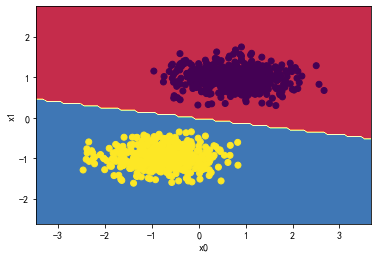
👉1、请参考LinearSVC.pdf文档，将莺尾花的数据替换为make_blobs自动生成两个测试数据集（一个是两个类别数据完全分离，另一个是两个类别数据有很少部分的交叉），对比KNN，贝叶斯，决策树，随机森林还有LinearSVC的分界边界线的区别。

（1）数据完全分离
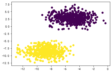
数据：

X,y = datasets.make_blobs(n_samples=1000, n_features=2, centers=2, cluster_std=1.5)
plt.scatter(X[:,0],X[:,1],c=y)
plt.show()

KNN：

knn_classifier = KNeighborsClassifier(n_neighbors=5)
knn_classifier.fit(X_standard, y)
plot_decision_boundary(knn_classifier,X_standard,y)

贝叶斯：

from sklearn.naive_bayes import GaussianNB
Gaussian_classifier = GaussianNB()
Gaussian_classifier.fit(X_standard, y)
plot_decision_boundary(Gaussian_classifier,X_standard, y)

决策树：

from sklearn.tree import DecisionTreeClassifier
DTree_classifier = DecisionTreeClassifier(max_depth=3)
DTree_classifier.fit(X_standard, y)
plot_decision_boundary(DTree_classifier,X_standard, y)

随机森林：

from sklearn.ensemble import RandomForestClassifier
random_forest = RandomForestClassifier(n_estimators=500)
random_forest.fit(X_standard, y)
plot_decision_boundary(random_forest,X_standard, y)

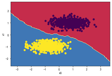
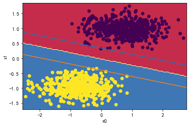
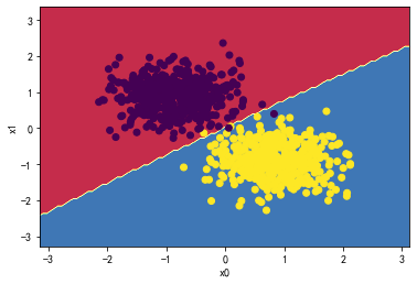
LinearSVC：

from sklearn.svm import LinearSVC
svc = LinearSVC()
svc.fit(X_standard, y)
plot_decision_boundary(svc,X_standard, y)

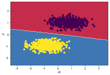
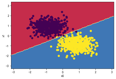
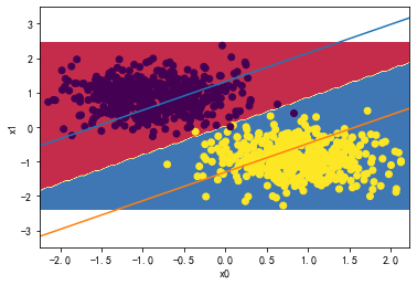
svc = LinearSVC(C=0.01)
svc.fit(X_standard, y)
plot_svc_decision_boundary(svc,X_standard, y)
svc.coef_

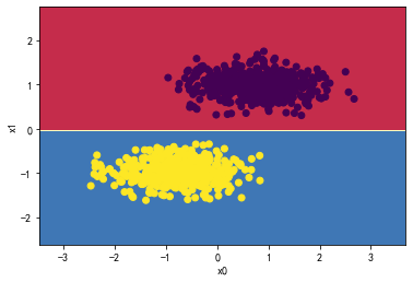
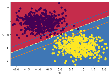
svc = LinearSVC(C=30)
svc.fit(X_standard, y)
plot_svc_decision_boundary(svc,X_standard, y)
svc.coef_

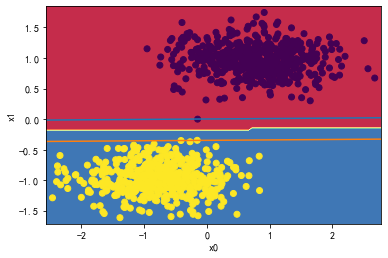
svc = LinearSVC(C=1000)
svc.fit(X_standard1, y)
plot_svc_decision_boundary(svc,X_standard1, y)

（2）数据部分交叉：
数据：

X,y = datasets.make_blobs(n_samples=1000, n_features=2, centers=2, cluster_std=1.5)
plt.scatter(X[:,0],X[:,1],c=y)
plt.show()

KNN：

knn_classifier = KNeighborsClassifier(n_neighbors=5)
knn_classifier.fit(X_standard, y)
plot_decision_boundary(knn_classifier,X_standard,y)

贝叶斯：

from sklearn.naive_bayes import GaussianNB
Gaussian_classifier = GaussianNB()
Gaussian_classifier.fit(X_standard, y)
plot_decision_boundary(Gaussian_classifier,X_standard, y)

决策树：

from sklearn.tree import DecisionTreeClassifier
DTree_classifier = DecisionTreeClassifier(max_depth=3)
DTree_classifier.fit(X_standard, y)
plot_decision_boundary(DTree_classifier,X_standard, y)

随机森林：

from sklearn.ensemble import RandomForestClassifier
random_forest = RandomForestClassifier(n_estimators=500)
random_forest.fit(X_standard, y)
plot_decision_boundary(random_forest,X_standard, y)

LinearSVC：

from sklearn.svm import LinearSVC
svc = LinearSVC()
svc.fit(X_standard, y)
plot_decision_boundary(svc,X_standard, y)

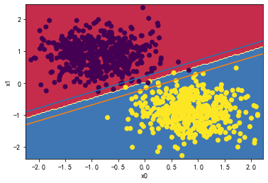
svc = LinearSVC(C=0.01)
svc.fit(X_standard, y)
plot_svc_decision_boundary(svc,X_standard, y)
svc.coef_

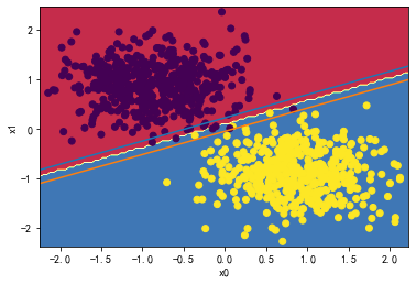
svc = LinearSVC(C=30)
svc.fit(X_standard, y)
plot_svc_decision_boundary(svc,X_standard, y)
svc.coef_

svc = LinearSVC(C=1000)
svc.fit(X_standard1, y)
plot_svc_decision_boundary(svc,X_standard1, y)

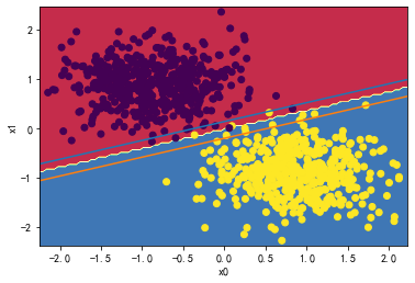
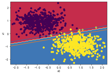
👉2、请详细测试LinearSVC中的C超参数对分类分界边界线的影响。

for i in [0.01,1,1000,10000000]:
    svc = LinearSVC(C=i)
    svc.fit(X_standard, y)
    plot_svc_decision_boundary(svc,X_standard, y)
    svc.coef_

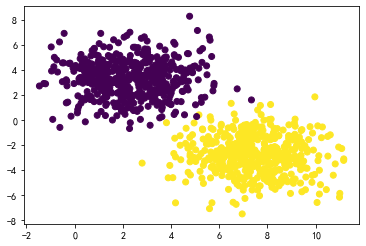
👉3、请同时对比，LinearSVC，NuSVC和SVC，三者在莺尾花数据集，make_blobs生成的数据集，还有makemoons生成的数据集，还有makecircles生成的数据集，对比差异。

（1）生成数据对比：

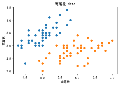
#↓莺尾花的数据集↓#
iris = datasets.load_iris()
#采用花瓣长宽
X = iris.data[0:100,:2]
y = iris.target[0:100]
plt.scatter(X[y==0,0],X[y==0,1])
plt.scatter(X[y==1,0],X[y==1,1])
plt.title('莺尾花 data')
plt.xlabel('花萼长')
plt.ylabel('花萼宽')
plt.show()

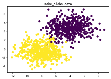
#↓make_blobs的数据集↓#
X,y = datasets.make_blobs(n_samples=1000, n_features=2, centers=2, cluster_std=1.5)
plt.title('make_blobs data')
plt.scatter(X[:,0],X[:,1],c=y)
plt.show()

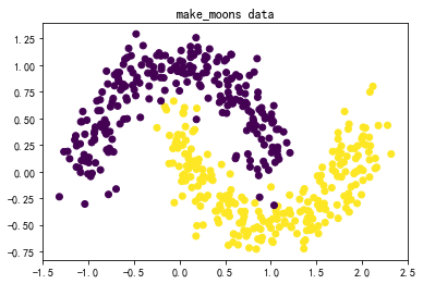
#↓makemoons的数据集↓#
X,y = datasets.make_moons(n_samples=500,noise=0.15)
plt.title('make_moons data')
plt.scatter(X[:,0],X[:,1],marker='o',c=y)
plt.show()

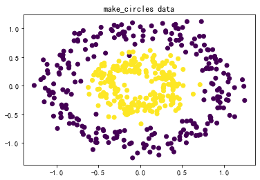
#↓makecircles的数据集↓#
X,y = datasets.make_circles(n_samples=500,factor=0.4,noise=0.12)
plt.title('make_circles data')
plt.scatter(X[:,0],X[:,1],marker='o',c=y)
plt.show()

（2）三种SVM分类方法和四组数据综合对比：
备注：三种分类方法纵向对比，四组数组横向对比
数据：图3-1 莺尾花数据、图3-2 make_blobs生成的数据、图3-3 makemoons生成的数据、图3-4 makecircles生成的数据。

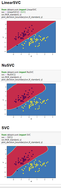
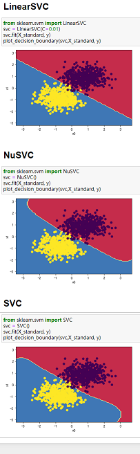
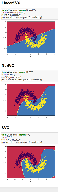
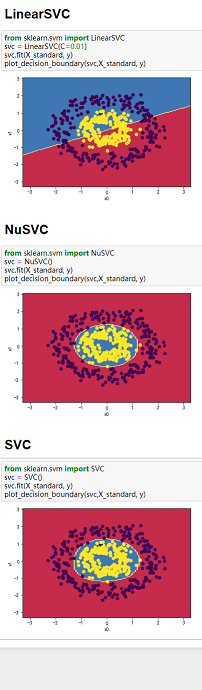
图3-1 图3-2 图3-3 图3-4

四、实验总结
       1、掌握了支持向量机的原理
       2、理解了支持向量机分类算法；
       3、掌握了sklearn的支持向量机分类算法；
       4、当数据分类界限明显且能用直线分割时，可以用LinearSVC；当数据类别分界线呈包围或者半包围状态时，用SVC最好。综上，SVC处理数据综合性最好。

五、附录
1、源码（注：空一行即jupyter notebook里一个可执行代码块）：

SVC实验5-1、2.ipynb

from sklearn import datasets
import matplotlib.pyplot as plt
import numpy as np
from sklearn.model_selection import train_test_split
from sklearn.neighbors import KNeighborsClassifier
from sklearn.metrics import accuracy_score
from warnings import simplefilter
simplefilter(action='ignore', category=FutureWarning)
plt.rcParams['font.sans-serif'] = ['SimHei']
plt.rcParams['axes.unicode_minus']=False # 用来正常显示负号

X,y = datasets.make_blobs(n_samples=1000, n_features=2, centers=2, cluster_std=1.5)
plt.scatter(X[:,0],X[:,1],c=y)
plt.show()

#X只有2个特征
def plot_decision_boundary(model, X, y):
    x0_min, x0_max = X[:,0].min()-1, X[:,0].max()+1
    x1_min, x1_max = X[:,1].min()-1, X[:,1].max()+1
    x0, x1 = np.meshgrid(np.linspace(x0_min, x0_max, 100), np.linspace(x1_min, x1_max, 100))
    Z = model.predict(np.c_[x0.ravel(), x1.ravel()])
    Z = Z.reshape(x0.shape)

    plt.contourf(x0, x1, Z, cmap=plt.cm.Spectral)
    plt.ylabel('x1')
    plt.xlabel('x0')
    plt.scatter(X[:, 0], X[:, 1], c=np.squeeze(y))
    plt.show()

#SVM数归一化，因为要算距离
from sklearn.preprocessing import StandardScaler
standardScaler = StandardScaler()
standardScaler.fit(X)
X_standard = standardScaler.transform(X)

knn_classifier = KNeighborsClassifier(n_neighbors=5)
knn_classifier.fit(X_standard, y)
plot_decision_boundary(knn_classifier,X_standard,y)

from sklearn.naive_bayes import GaussianNB
Gaussian_classifier = GaussianNB()
Gaussian_classifier.fit(X_standard, y)
plot_decision_boundary(Gaussian_classifier,X_standard, y)

from sklearn.tree import DecisionTreeClassifier
DTree_classifier = DecisionTreeClassifier(max_depth=3)
DTree_classifier.fit(X_standard, y)
plot_decision_boundary(DTree_classifier,X_standard, y)

from sklearn.ensemble import RandomForestClassifier
random_forest = RandomForestClassifier(n_estimators=500)
random_forest.fit(X_standard, y)
plot_decision_boundary(random_forest,X_standard, y)

from sklearn.svm import LinearSVC
svc = LinearSVC()
svc.fit(X_standard, y)
plot_decision_boundary(svc,X_standard, y)

svc = LinearSVC(C=0.01)
svc.fit(X_standard, y)
plot_decision_boundary(svc,X_standard, y)

svc.coef_

svc.intercept_

#svc上下边界图绘制，X只有2个特征
def plot_svc_decision_boundary(model, X, y):
    x0_min, x0_max = X[:,0].min()-0.1, X[:,0].max()+0.1
    x1_min, x1_max = X[:,1].min()-0.1, X[:,1].max()+0.1
    x0, x1 = np.meshgrid(np.linspace(x0_min, x0_max, 100), np.linspace(x1_min, x1_max, 100))
    Z = model.predict(np.c_[x0.ravel(), x1.ravel()])
    Z = Z.reshape(x0.shape)
    plt.contourf(x0, x1, Z, cmap=plt.cm.Spectral)
    plt.ylabel('x1')
    plt.xlabel('x0')
    plt.scatter(X[:, 0], X[:, 1], c=np.squeeze(y))
    w = model.coef_[0]
    b = model.intercept_[0]
    #w0*x0 + w1*x1 +b =0
    # x1 = -w0/w1*x0 - (b+1)/w1
    plot_x = np.linspace(x0_min,x0_max,200)
    up_y = -w[0]/w[1]*plot_x - (b+1)/w[1]
    dn_y = -w[0]/w[1]*plot_x - (b-1)/w[1]
    plt.plot(plot_x,up_y)
    plt.plot(plot_x,dn_y)
    plt.show()

svc = LinearSVC(C=i)
svc.fit(X_standard, y)
plot_svc_decision_boundary(svc,X_standard, y)
svc.coef_

np.sum(X_standard*svc.coef_+svc.intercept_,axis=1)

svc = LinearSVC(C=30)
svc.fit(X_standard, y)
plot_svc_decision_boundary(svc,X_standard, y)
svc.coef_

X_standard1= X_standard.copy()
X_standard1[1,:]=np.array([-0.15,0])

svc = LinearSVC(C=1000)
svc.fit(X_standard1, y)
plot_svc_decision_boundary(svc,X_standard1, y)

SVC实验5-3.ipynb

from sklearn import datasets
import matplotlib.pyplot as plt
import numpy as np
from sklearn.model_selection import train_test_split
from sklearn.neighbors import KNeighborsClassifier
from sklearn.metrics import accuracy_score
from warnings import simplefilter
simplefilter(action='ignore', category=FutureWarning)
plt.rcParams['font.sans-serif'] = ['SimHei']
plt.rcParams['axes.unicode_minus']=False # 用来正常显示负号

iris = datasets.load_iris()
##采用花瓣长宽
X = iris.data[0:100,:2]
y = iris.target[0:100]
plt.scatter(X[y==0,0],X[y==0,1])
plt.scatter(X[y==1,0],X[y==1,1])
plt.title('莺尾花 data')
plt.xlabel('花萼长')
plt.ylabel('花萼宽')
plt.show()

X,y = datasets.make_blobs(n_samples=1000, n_features=2, centers=2, cluster_std=1.5)
plt.title('make_blobs data')
plt.scatter(X[:,0],X[:,1],c=y)
plt.show()

X,y = datasets.make_moons(n_samples=500,noise=0.15)
plt.title('make_moons data')
plt.scatter(X[:,0],X[:,1],marker='o',c=y)
plt.show()

X,y = datasets.make_circles(n_samples=500,factor=0.4,noise=0.12)
plt.title('make_circles data')
plt.scatter(X[:,0],X[:,1],marker='o',c=y)
plt.show()

#X只有2个特征
def plot_decision_boundary(model, X, y):
    x0_min, x0_max = X[:,0].min()-1, X[:,0].max()+1
    x1_min, x1_max = X[:,1].min()-1, X[:,1].max()+1
    x0, x1 = np.meshgrid(np.linspace(x0_min, x0_max, 100), np.linspace(x1_min, x1_max, 100))
    Z = model.predict(np.c_[x0.ravel(), x1.ravel()])
    Z = Z.reshape(x0.shape)

    plt.contourf(x0, x1, Z, cmap=plt.cm.Spectral)
    plt.ylabel('x1')
    plt.xlabel('x0')
    plt.scatter(X[:, 0], X[:, 1], c=np.squeeze(y))
    plt.show()

#SVM数归一化，因为要算距离
from sklearn.preprocessing import StandardScaler
standardScaler = StandardScaler()
standardScaler.fit(X)
X_standard = standardScaler.transform(X)

from sklearn.svm import LinearSVC
svc = LinearSVC(C=0.01)
svc.fit(X_standard, y)
plot_decision_boundary(svc,X_standard, y)

from sklearn.svm import NuSVC
svc = NuSVC()
svc.fit(X_standard, y)
plot_decision_boundary(svc,X_standard, y)

from sklearn.svm import SVC
svc = SVC()
svc.fit(X_standard, y)
plot_decision_boundary(svc,X_standard, y)

鄙人第一次写博客，（写着玩玩记录一下）
end

posted @ 2020-11-23 22:59 灰小k 阅读(1341) 评论(0) 收藏举报

刷新页面返回顶部

灰小k

为触礁的船只祈祷，做自己的灯塔。

实验5 支持向量机分类实验

公告