
Python小练习:线性衰减
作者:凯鲁嘎吉 - 博客园 http://www.cnblogs.com/kailugaji/
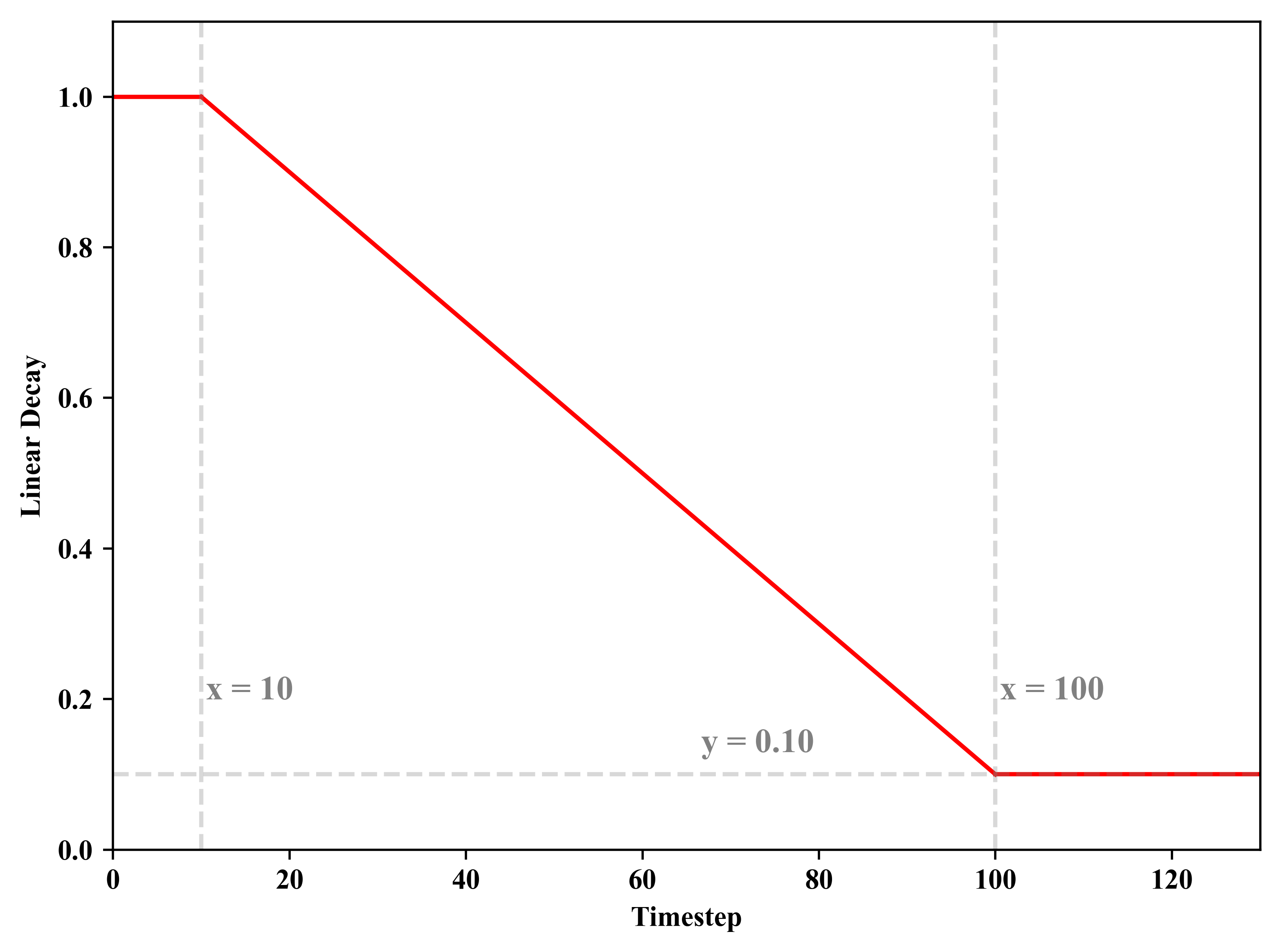
本文介绍一种最简单的衰减曲线:线性衰减。给定schedule = [start, end, start_value, end_value],先前一直保持在start_value水平,从start时刻开始衰减,直至到达end时刻结束,其值为end_value,之后就一直保持在end_value这一水平上不变。
1. get_scheduled_value_test.py
 1 # -*- coding: utf-8 -*-
 2 # Author:凯鲁嘎吉 Coral Gajic
 3 # https://www.cnblogs.com/kailugaji/
 4 # Python小练习:线性衰减
 5 import numpy as np
 6 import matplotlib.pyplot as plt
 7 plt.rc('font',family='Times New Roman')
 8 # Scheduled Exploration Noise
 9 # linear decay
10 def get_scheduled_value(current, schedule):
11     start, end, start_value, end_value = schedule
12     ratio = (current - start) / (end - start) # 当前步数在总步数的比例
13     # 总计100步,当前current步
14     ratio = max(0, min(1, ratio))
15     value = (ratio * (end_value - start_value)) + start_value
16     return value
17
18 start = 10 # 从这时开始衰减
19 end = 100 # the decay horizon
20 start_value = 1 # 从1衰减到0.1
21 end_value = 0.1
22 schedule = [start, end, start_value, end_value]
23 exploration_noise = []
24 for i in range(int(end - start)+1):
25     value = get_scheduled_value(start + i, schedule)
26     exploration_noise.append(value)
27
28 # --------------------画图------------------------
29 # 手动设置横纵坐标范围
30 plt.xlim([0, end*1.3])
31 plt.ylim([0, start_value + 0.1])
32 my_time = np.arange(start, end+1)
33 exploration_noise = np.array(exploration_noise)
34 plt.plot([0, start], [start_value, start_value], color = 'red', ls = '-')
35 plt.plot(my_time, exploration_noise, color = 'red', ls = '-')
36 plt.plot([end, end*1.3], [end_value, end_value], color = 'red', ls = '-')
37 # 画3条不起眼的虚线
38 plt.plot([0, end*1.3], [exploration_noise[-1], exploration_noise[-1]], color = 'gray', ls = '--', alpha = 0.3)
39 plt.text(end - end/3, exploration_noise[-1] + 0.03, "y = %.2f" %exploration_noise[-1], fontdict={'size': '12', 'color': 'gray'})
40 plt.plot([start, start], [0, start_value + 0.1], color = 'gray', ls = '--', alpha = 0.3)
41 plt.text(start + 0.5, start_value - 0.8, "x = %d" %start, fontdict={'size': '12', 'color': 'gray'})
42 plt.plot([end, end], [0, start_value + 0.1], color = 'gray', ls = '--', alpha = 0.3)
43 plt.text(end + 0.5, start_value - 0.8, "x = %d" %end, fontdict={'size': '12', 'color': 'gray'})
44 # 横纵坐标轴
45 plt.xlabel('Timestep')
46 plt.ylabel('Linear Decay')
47 plt.tight_layout()
48 plt.savefig('Linear Decay.png', bbox_inches='tight', dpi=500)
49 plt.show()
2. 结果
3. 参考文献
[1] Yarats D, Fergus R, Lazaric A, et al. Mastering visual continuous control: Improved data-augmented reinforcement learning[J]. arXiv preprint arXiv:2107.09645, 2021.

 浙公网安备 33010602011771号