Python小练习：Sinkhorn-Knopp算法

Python小练习：Sinkhorn-Knopp算法

作者：凯鲁嘎吉 - 博客园 http://www.cnblogs.com/kailugaji/

本文介绍Sinkhorn-Knopp算法的Python实现，通过参考并修改两种不同的实现方法，来真正弄懂算法原理。详细的原理部分可参考文末给出的参考文献。
公式为：$P = diag(u)\exp \left( {\frac{{ - S}}{\varepsilon }} \right)diag(v)$。输入S，输出P，其中u与v是renormalization向量，eps用来控制P的平滑性。通常情况下，S与P对应的值成反比，S某一元素越大，相应的P值越小。

1. sinkhorn_test.py

# -*- coding: utf-8 -*-
# Author：凯鲁嘎吉 Coral Gajic
# https://www.cnblogs.com/kailugaji/
# Sinkhorn-Knopp算法(以方阵为例)
# 对于一个n*n方阵
# 1) 先逐行做归一化：将第一行的每个元素除以第一行所有元素之和，得到新的"第一行"，每行都做相同的操作
# 2) 再逐列做归一化，操作同上
# 重复以上的两步1)与2)，最终可以收敛到一个行和为1，列和也为1的双随机矩阵。
import torch
import numpy as np
import time
import seaborn as sns
import matplotlib.pyplot as plt
# 方法1：
'''
    https://github.com/miralab-ustc/rl-cbm
'''
# numpy转换成tensor
def sinkhorn(scores, eps = 5, n_iter = 3):
    def remove_infs(x): # 替换掉数据里面的INF与0
        mm = x[torch.isfinite(x)].max().item() # m是x的最大值
        x[torch.isinf(x)] = mm # 用最大值替换掉数据里面的INF
        x[x==0] = 1e-38 # 将数据里面的0元素替换为1e-38
        return x
    # 若以(2, 8)为例
    scores = torch.tensor(scores)
    t0 = time.time()
    n, m = scores.shape # torch.Size([2, 8])
    scores1 = scores.view(n*m) # torch.Size([16])
    Q = torch.softmax(-scores1/eps, dim=0) # softmax
    Q = remove_infs(Q).view(n,m).T # torch.Size([8, 2])
    r, c = torch.ones(n), torch.ones(m) * (n / m)
    # 确保sum(r)=sum(c)
    # 对应地P的行和为r，列和为c
    for _ in range(n_iter):
        u = (c/torch.sum(Q, dim=1)) # torch.sum(Q, dim=1)按列求和，得到1行8列的数torch.Size([8])
        Q *= remove_infs(u).unsqueeze(1) #  torch.Size([8, 2])
        v = (r/torch.sum(Q,dim=0)) # torch.sum(Q,dim=0)按行求和，得到torch.Size([2])
        Q *= remove_infs(v).unsqueeze(0) # torch.Size([8, 2])
    bsum = torch.sum(Q, dim=0, keepdim=True) # 按行求和，torch.Size([1, 2])
    Q = Q / remove_infs(bsum)
    # bsum = torch.sum(Q, dim=1, keepdim=True)
    # Q = Q / remove_infs(bsum)
    P = Q.T # 转置，torch.Size([2, 8])
    t1 = time.time()
    compute_time = t1 - t0
    assert torch.isnan(P.sum())==False
    P = np.array(P)
    scores = np.array(scores)
    dist = np.sum(P * scores)
    return P, dist, compute_time

# 方法2：
# Sinkhorn-Knopp算法
'''
    https://michielstock.github.io/posts/2017/2017-11-5-OptimalTransport/
    https://zhuanlan.zhihu.com/p/542379144
'''
# numpy
def compute_optimal_transport(scores, eps = 5, n_iter = 3):
    """
    Computes the optimal transport matrix and Sinkhorn distance using the
    Sinkhorn-Knopp algorithm
    Inputs:
        - scores : cost matrix (n * m)
        - r : vector of marginals (n, )
        - c : vector of marginals (m, )
        - eps : strength of the entropic regularization
        - epsilon : convergence parameter
    Outputs:
        - P : optimal transport matrix (n x m)
        - dist : Sinkhorn distance
    """
    t0 = time.time()
    n, m = scores.shape
    r = np.ones(n)  # P矩阵列和为r
    c = np.ones(m)*(n/m)  # P矩阵行和为c
    # 确保：np.sum(r)==np.sum(c)
    P = np.exp(- scores / eps)
    P /= P.sum()
    u = np.zeros(n)
    # normalize this matrix
    # while np.max(np.abs(u - P.sum(1))) > epsilon:
    for _ in range(n_iter):
        u = P.sum(1)
        P *= (r / u).reshape((-1, 1)) # 行归r化
        P *= (c / P.sum(0)).reshape((1, -1)) # 列归c化
    t1 = time.time()
    compute_time = t1 - t0
    dist = np.sum(P * scores)
    return P, dist, compute_time

np.random.seed(1)
n = 5 # 行数
m = 5 # 列数
num = 3 # 保留小数位数
n_iter = 100 # 迭代次数
eps = 0.5
scores = np.random.rand(n ,m) # cost matrix
print('原始数据：\n', np.around(scores, num))
print('------------------------------------------------')
# 方法1：
P, dist, compute_time_1 = sinkhorn(scores, eps = eps, n_iter = n_iter)
print('1. 处理后的结果：\n', np.around(P, num))
print('1. 行和：\n', np.sum(P, axis = 0))
print('1. 列和：\n', np.sum(P, axis = 1))
print('1. Sinkhorn距离：', np.around(dist, num))
print('1. 计算时间：', np.around(compute_time_1, 8), '秒')
print('------------------------------------------------')
# 方法2：
P, dist, compute_time_2 = compute_optimal_transport(scores, eps = eps, n_iter = n_iter)
print('2. 处理后的结果：\n', np.around(P, num))
print('2. 行和：\n', np.sum(P, axis = 0))
print('2. 列和：\n', np.sum(P, axis = 1))
print('2. Sinkhorn距离：', np.around(dist, num))
print('2. 计算时间：', np.around(compute_time_2, 8), '秒')
if True:
    # 绘制热力图
    fig, ax = plt.subplots(1, 2, figsize=(15, 7))
    for axs in ax:
        axs.tick_params(labelsize=15)
    sns.set(font_scale=1.5, font='Times New Roman')
    sns.heatmap(scores, ax=ax[0], cmap = 'Blues')
    sns.heatmap(P, ax=ax[1], cmap = 'Blues')
    plt.rcParams['font.sans-serif'] = ['KaiTI']
    plt.rcParams['axes.unicode_minus'] = False
    ax[0].set_title("原始数据", fontsize=20)
    ax[1].set_title("处理后的数据", fontsize=20)
    plt.tight_layout()
    plt.savefig("confusion_matrix.png", dpi = 500)
    plt.show()

2. 结果

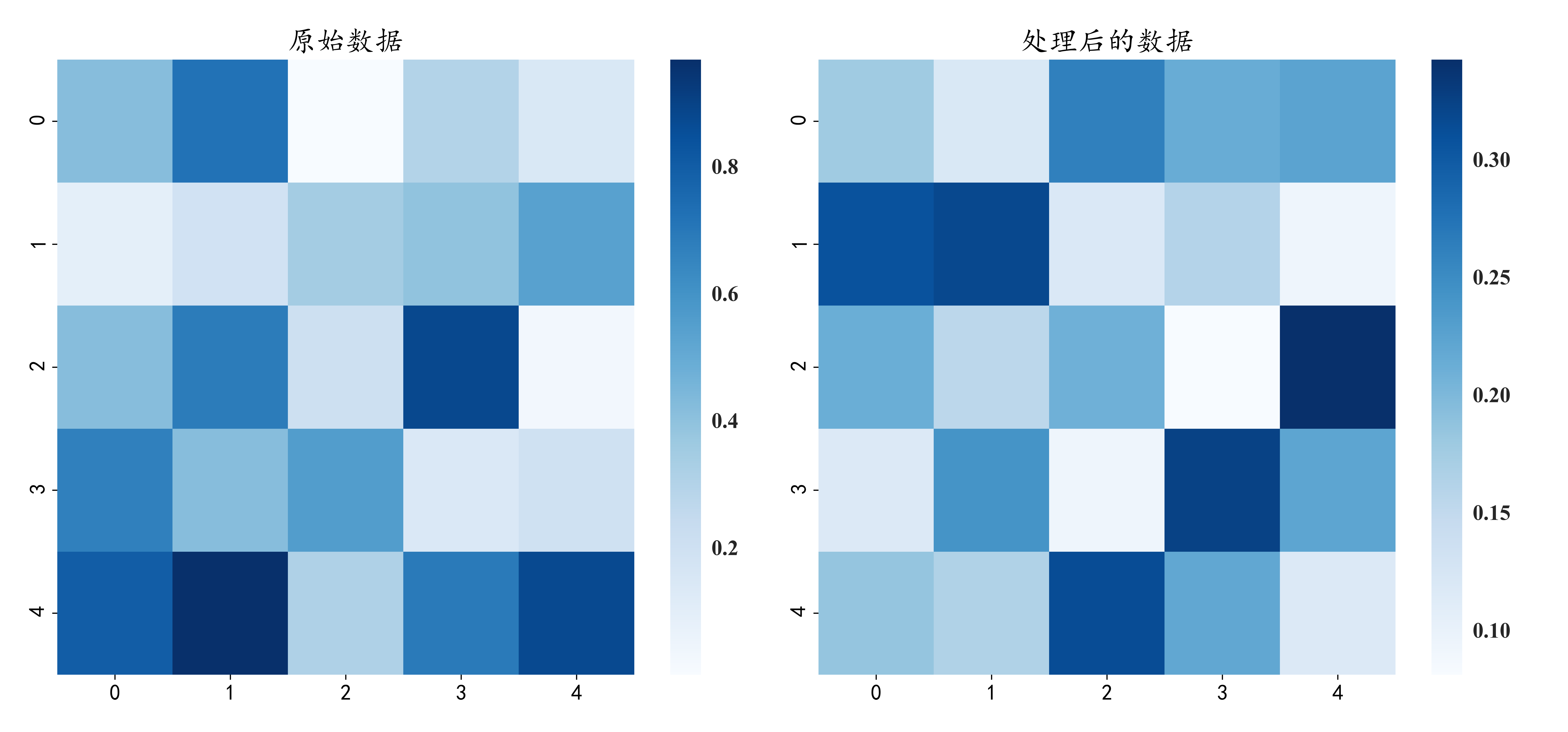
D:\ProgramData\Anaconda3\python.exe "D:/Python code/2023.3 exercise/Sinkhorn-Knopp算法/sinkhorn_test.py"
原始数据：
 [[0.417 0.72  0.    0.302 0.147]
 [0.092 0.186 0.346 0.397 0.539]
 [0.419 0.685 0.204 0.878 0.027]
 [0.67  0.417 0.559 0.14  0.198]
 [0.801 0.968 0.313 0.692 0.876]]
------------------------------------------------
1. 处理后的结果：
 [[0.178 0.121 0.263 0.214 0.225]
 [0.308 0.318 0.119 0.161 0.093]
 [0.212 0.155 0.209 0.081 0.342]
 [0.117 0.242 0.094 0.324 0.222]
 [0.185 0.164 0.314 0.22  0.117]]
1. 行和：
 [1. 1. 1. 1. 1.]
1. 列和：
 [1. 1. 1. 1. 1.]
1. Sinkhorn距离： 1.802
1. 计算时间： 0.01741338 秒
------------------------------------------------
2. 处理后的结果：
 [[0.178 0.121 0.263 0.214 0.225]
 [0.308 0.318 0.119 0.161 0.093]
 [0.212 0.155 0.209 0.081 0.342]
 [0.117 0.242 0.094 0.324 0.222]
 [0.185 0.164 0.314 0.22  0.117]]
2. 行和：
 [1. 1. 1. 1. 1.]
2. 列和：
 [1. 1. 1. 1. 1.]
2. Sinkhorn距离： 1.802
2. 计算时间： 0.00100136 秒

Process finished with exit code 0

热力图：

当 n=10, m=5 时，结果为

D:\ProgramData\Anaconda3\python.exe "D:/Python code/2023.3 exercise/sinkhorn_test.py"
原始数据：
 [[0.417 0.72  0.    0.302 0.147]
 [0.092 0.186 0.346 0.397 0.539]
 [0.419 0.685 0.204 0.878 0.027]
 [0.67  0.417 0.559 0.14  0.198]
 [0.801 0.968 0.313 0.692 0.876]
 [0.895 0.085 0.039 0.17  0.878]
 [0.098 0.421 0.958 0.533 0.692]
 [0.316 0.687 0.835 0.018 0.75 ]
 [0.989 0.748 0.28  0.789 0.103]
 [0.448 0.909 0.294 0.288 0.13 ]]
------------------------------------------------
1. 处理后的结果：
 [[0.17  0.111 0.299 0.183 0.237]
 [0.308 0.306 0.141 0.143 0.102]
 [0.2   0.141 0.234 0.068 0.356]
 [0.118 0.234 0.112 0.29  0.246]
 [0.177 0.152 0.358 0.188 0.124]
 [0.063 0.385 0.268 0.231 0.053]
 [0.422 0.265 0.058 0.151 0.104]
 [0.268 0.153 0.072 0.415 0.091]
 [0.082 0.16  0.259 0.105 0.393]
 [0.191 0.091 0.199 0.225 0.293]]
1. 行和：
 [2. 2. 2. 2. 2.]
1. 列和：
 [1. 1. 1. 1. 1. 1. 1. 1. 1. 1.]
1. Sinkhorn距离： 3.356
1. 计算时间： 0.02233005 秒
------------------------------------------------
2. 处理后的结果：
 [[0.17  0.111 0.299 0.183 0.237]
 [0.308 0.306 0.141 0.143 0.102]
 [0.2   0.141 0.234 0.068 0.356]
 [0.118 0.234 0.112 0.29  0.246]
 [0.177 0.152 0.358 0.188 0.124]
 [0.063 0.385 0.268 0.231 0.053]
 [0.422 0.265 0.058 0.151 0.104]
 [0.268 0.153 0.072 0.415 0.091]
 [0.082 0.16  0.259 0.105 0.393]
 [0.191 0.091 0.199 0.225 0.293]]
2. 行和：
 [2. 2. 2. 2. 2.]
2. 列和：
 [1. 1. 1. 1. 1. 1. 1. 1. 1. 1.]
2. Sinkhorn距离： 3.356
2. 计算时间： 0.00100446 秒

Process finished with exit code 0

热力图：

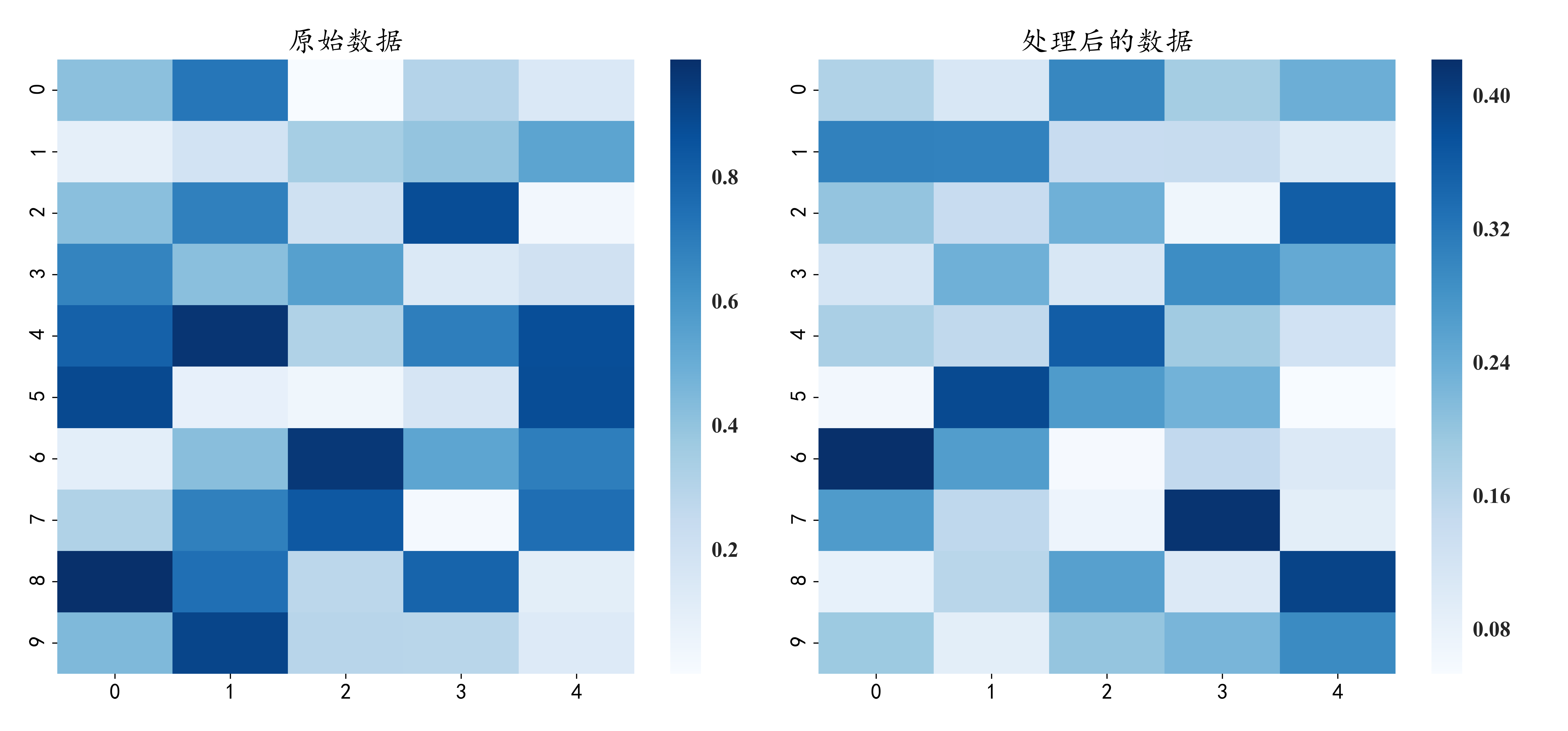
从热力图中也可以看出左边颜色深的块到了右边对应位置，颜色就成了浅色，说明S与P成反比。

3. 参考文献

[1] Cuturi M. Sinkhorn distances: Lightspeed computation of optimal transport[C]. NIPS, 2013.
[2] Liu Q, Zhou Q, Yang R, et al. Robust Representation Learning by Clustering with Bisimulation Metrics for Visual Reinforcement Learning with Distractions[C]. AAAI, 2023.
[3] Michiel Stock, Notes on Optimal Transport, https://michielstock.github.io/posts/2017/2017-11-5-OptimalTransport/

[4] 最优传输问题（Optimal Transport Problem） -  套娃的套娃 - 知乎