前言
尽管R语言中诸如ggpubr等包为统计学可视化提供了便捷的函数,但在实际应用中,问题往往并不那么简单。这些包通常仅支持简单的两组对比或全局检验,虽然能够快速生成初步结果,却无法帮助用户判断统计方法选择的合理性,也难以直接生成符合发表要求的统计学结果。
在高质量的SCI期刊中,统计学编辑或审稿人通常会对文章中每一个数据的统计方法和结果进行严格审查。统计学编辑拥有一票否决权,即使学术审稿人对你的研究给予了高度评价,一旦统计方法存在问题且无法满足修改要求,你的文章仍可能面临无情的拒稿。
为解决这一问题,我在多方探索和汇总的基础上,结合专业统计学老师的指导,整理了一份适用于多分组统计检验的代码,供读者参考。当然,为了提高泛用性,我也在流程中补充了两组间分析的内容。由于我并非统计学专业出身,且受限于课题需求,提供的代码可能存在一定的局限性,也不会适用所有情况。本文的主要目的是抛砖引玉,希望读者能够根据自身实际需求,形成适合的工作流程。
事实上,最重要的仍然是对统计学知识的正确认知,才能帮助你做出正确的选择,任何既定的流程都是辅助。对于统计学方法选择,我认为这一篇推文已经足够解释清楚:
https://mp.weixin.qq.com/s/IF4F0W2ghWRq4ILVP3T49A
为降低阅读难度,我将统计函数封装为一个脚本,并附上了我自用的简单绘图脚本。本文以梳理多分组统计检验的工作流程和结果解读为核心,旨在帮助读者从头构建完整的分析流程。如果读者对封装的流程感兴趣,可以自行拆解和改编内容。
参考数据和函数
从github页面获取:https://github.com/Doctorluka/Multiple_Group_Statistics
示例数据:来自GraphPad Prism的two-way anova测试数据
函数:
stat_test.R用于统计stat_plot.R用于简单绘图
工作流程图:
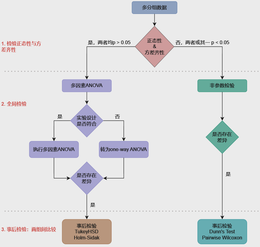
主函数和子函数简介
| 主函数 | 说明 | 二级函数 | 三级函数 |
|---|---|---|---|
| test_assumptions | 正态性与方差齐性检验 | perform_shapiro_by_group perform_variances_homogeneity_test | |
| auto_stat_test | 自动全局检验和事后检验 | perform_anova_test perform_kw_test perfrom_stat_for_two_group | build_aov_formula preform_avo_post_hoc perform_pairwise_wilcoxon rev_dunn_comparision |
| stat_res_collect stat_res_collect_two_group | 数据整理 | p_to_stars |
函数使用
1. 首先我们新建一个R project,并进入工作目录,通常我会在工作目录下创建以下文件夹
.
├── data        # 原始数据
├── figures     # 绘图
├── test.Rproj
├── results     # 输出
├── scripts     # 脚本
└── utils       # 存放当前项目使用的封装函数
2. 导入必要的R包和函数
suppressPackageStartupMessages({
  library(openxlsx)
  library(tibble)
  library(tidyverse)
  library(ggpubr)
  source("utils/stat_test.R")
  source("utils/stat_plot.R")
})
3. 读入数据。
这是graphpad prism的双因素方差分析的示例数据,主要包括两个干预因素:某基因的敲除(KO vs. WT)和不同培养条件(Serum_starved vs. Normal_culture)下检测的某项指标。
group列为分组,value列为检测指标的值。
实验设计为典型的两两组合设计,符合双因素方差分析的需求。
test_data <- read.xlsx("data/test.xlsx")
#                group value
# 1   WT_Serum_starved    34
# 2   WT_Serum_starved    36
# 3   WT_Serum_starved    41
# 4   WT_Serum_starved    43
# 5   KO_Serum_starved    98
# 6   KO_Serum_starved    87
# 7   KO_Serum_starved    95
# 8   KO_Serum_starved    99
# 9   KO_Serum_starved    88
# 10 WT_Normal_culture    23
# 11 WT_Normal_culture    19
# 12 WT_Normal_culture    26
# 13 WT_Normal_culture    29
# 14 WT_Normal_culture    25
# 15 KO_Normal_culture    32
# 16 KO_Normal_culture    29
# 17 KO_Normal_culture    26
# 18 KO_Normal_culture    33
# 19 KO_Normal_culture    30
4. 为数据加入干预因素的标记
test_data$ko <- ifelse(test_data$group %in% c("WT_Serum_starved", "WT_Normal_culture"), "no", "yes")
test_data$culture <- ifelse(test_data$group %in% c("WT_Serum_starved", "KO_Serum_starved"), "Serum_starved", "Normal_culture")

#                group value  ko        culture
# 1   WT_Serum_starved    34  no  Serum_starved
# 2   WT_Serum_starved    36  no  Serum_starved
# 3   WT_Serum_starved    41  no  Serum_starved
# 4   WT_Serum_starved    43  no  Serum_starved
# 5   KO_Serum_starved    98 yes  Serum_starved
# 6   KO_Serum_starved    87 yes  Serum_starved
# 7   KO_Serum_starved    95 yes  Serum_starved
# 8   KO_Serum_starved    99 yes  Serum_starved
# 9   KO_Serum_starved    88 yes  Serum_starved
# 10 WT_Normal_culture    23  no Normal_culture
# 11 WT_Normal_culture    19  no Normal_culture
# 12 WT_Normal_culture    26  no Normal_culture
# 13 WT_Normal_culture    29  no Normal_culture
# 14 WT_Normal_culture    25  no Normal_culture
# 15 KO_Normal_culture    32 yes Normal_culture
# 16 KO_Normal_culture    29 yes Normal_culture
# 17 KO_Normal_culture    26 yes Normal_culture
# 18 KO_Normal_culture    33 yes Normal_culture
# 19 KO_Normal_culture    30 yes Normal_culture
5. 检测正态性与方差齐性
使用参数说明:
data:输入数据,需要为“清洁数据”,即同一指标的连续型/分类变量归为一列response_col:需要检测的数据的列名(此处为value)group_col:分组信息的列名(此处为group)method(optional):方差齐性检验的方法,默认为"levene",还可以选择"bartlett"。
nor_res <- test_assumptions(data = test_data, response_col = "value", group_col = "group", method = "levene")
# Finish shapiro.test!
# Finish levene test!
# Warning message:
# In leveneTest.default(y = y, group = group, ...) : group coerced to factor.
查看一下数据
输出结果为
list结构:
test.results:- step:标记这一步的意义,同样的步骤(例如正态性检验)有多个结果时,只标记一次
- method:对应step使用的统计学方法
- group:分组。正态性检验按照分开各组独立检验;而方差齐性则是检验各组之间的方差是否相等,标记为使用公式
- p.value:统计结果
- sig:显著性标记。如果存在p<0.05,则以
*标记。最高为****代表p<0.0001。
pass:TRUE代表同时符合正态性和方差齐性;FALSE代表正态性和方差齐性两者或其一不符合。
$test.results
                      step       method             group   p.value sig
1                Normality shapiro.test KO_Normal_culture 0.8326528
2                          shapiro.test  KO_Serum_starved 0.2359466
3                          shapiro.test WT_Normal_culture 0.9554189
4                          shapiro.test  WT_Serum_starved 0.5887706
5 Homogeneity of Variances   leveneTest     value ~ group 0.4012227

$pass
[1] TRUE
6. 全局检验和事后检验
进行正态性检验后,应该选择合适的检验方法。这里提供了自动选择的函数。
使用参数说明(与上面重复的参数不作说明):
test_assumptions_res:正态性与方差齐性检验结果,即上面的nor_res
factors:实验设计中的干预因素对应的列名,这里为c("ko", "culture")
interaction:是否考虑干预因素之间的交互效应,默认为TRUE
aov_post_hoc:ANOVA的事后检验方法,默认为holm,可选tukey
kw_post_hoc:KW的事后检验方法,默认为dunn,可选wilcox(任何非dunn的输入都会自动转为wilcox)
【备注】统计学老师告诉我,wilcoxon.test只有在没得选的时候才使用,并不是一种严谨的统计学方法,非必要不使用。
执行后,会自动打印检验信息。如果你的设计不符合two-way ANOVA,例如缺少了其中一组,则interaction无法计算,会自动转为one-way ANOVA,仅考虑group_col的主效应。
在这里,我们能看到ko和culture都具有显著性,且两者的交互作用ko:culture也是具有显著性。如果全局检验没有显著性,则会跳过事后检验步骤,并结束计算。
stat_res <- auto_stat_test(data = test_data,
                           test_assumptions_res = nor_res,
                           response_col = "value",
                           group_col = "group",
                           factors = c("ko", "culture"),
                           interaction = TRUE,
                           aov_post_hoc = "holm",
                           kw_post_hoc = "dunn")

# Normality and homogeneity of variances assumptions are met.
# Performing parametric test: ANOVA.
# Try to perform ANOVA test ...
# ---> Formula = value ~ ko*culture
# ANOVA results:
#             Df Sum Sq Mean Sq F value           Pr(>F)
# ko           1   4562    4562   259.8 0.00000000007008 ***
# culture      1   7631    7631   434.6 0.00000000000173 ***
# ko:culture   1   2859    2859   162.8 0.00000000185783 ***
# Residuals   15    263      18
# ---
# Signif. codes:  0 ‘***’ 0.001 ‘**’ 0.01 ‘*’ 0.05 ‘.’ 0.1 ‘ ’ 1
# ANOVA p<0.05. Performing post-hoc: holm.
#                            comparison               p.value     method
# 1  KO_Serum_starved-KO_Normal_culture 0.0000000000011615406 Holm-Sidak
# 2 WT_Normal_culture-KO_Normal_culture 0.0517738262855162654 Holm-Sidak
# 3  WT_Serum_starved-KO_Normal_culture 0.0170968348865750026 Holm-Sidak
# 4  WT_Normal_culture-KO_Serum_starved 0.0000000000004027528 Holm-Sidak
# 5   WT_Serum_starved-KO_Serum_starved 0.0000000000178067761 Holm-Sidak
# 6  WT_Serum_starved-WT_Normal_culture 0.0004606831583011530 Holm-Sidak
7. 数据整合和清洁
为了更加符合文章发表的需求,这里还提供了一个函数,用于整理上述数据并方便导出。
nor:为正态性与方差齐性检验结果
stat:为全局检验与事后检验结果
tast_name:该数据的名称(方便记录和查看)
stat_summary <- stat_res_collect(data = test_data, nor = nor_res, stat = stat_res, task_name = "demo_data")
# Complete data cleaning!
查看数据结构,为list结构:
demo_data:该命名源自tast_name参数,储存纳入统计的数据
stat_test:为上述两步的结果整合,具体内容可参考正态性与方差齐性的结果解读。
$demo_data
               group value  ko        culture
1   WT_Serum_starved    34  no  Serum_starved
2   WT_Serum_starved    36  no  Serum_starved
3   WT_Serum_starved    41  no  Serum_starved
4   WT_Serum_starved    43  no  Serum_starved
5   KO_Serum_starved    98 yes  Serum_starved
6   KO_Serum_starved    87 yes  Serum_starved
7   KO_Serum_starved    95 yes  Serum_starved
8   KO_Serum_starved    99 yes  Serum_starved
9   KO_Serum_starved    88 yes  Serum_starved
10 WT_Normal_culture    23  no Normal_culture
11 WT_Normal_culture    19  no Normal_culture
12 WT_Normal_culture    26  no Normal_culture
13 WT_Normal_culture    29  no Normal_culture
14 WT_Normal_culture    25  no Normal_culture
15 KO_Normal_culture    32 yes Normal_culture
16 KO_Normal_culture    29 yes Normal_culture
17 KO_Normal_culture    26 yes Normal_culture
18 KO_Normal_culture    33 yes Normal_culture
19 KO_Normal_culture    30 yes Normal_culture

$stat_test
        task                     step       method                               group p.value  sig
1  demo_data                Normality shapiro.test                   KO_Normal_culture  0.8327
2                                     shapiro.test                    KO_Serum_starved  0.2359
3                                     shapiro.test                   WT_Normal_culture  0.9554
4                                     shapiro.test                    WT_Serum_starved  0.5888
5            Homogeneity of Variances   leveneTest                       value ~ group  0.4012
6                    Parametric tests        ANOVA                         ko          <0.0001 ****
7                                                                          culture     <0.0001 ****
8                                                                          ko:culture  <0.0001 ****
9                       Post hoc test   Holm-Sidak  KO_Serum_starved-KO_Normal_culture <0.0001 ****
10                                      Holm-Sidak WT_Normal_culture-KO_Normal_culture  0.0518
11                                      Holm-Sidak  WT_Serum_starved-KO_Normal_culture  0.0171    *
12                                      Holm-Sidak  WT_Normal_culture-KO_Serum_starved <0.0001 ****
13                                      Holm-Sidak   WT_Serum_starved-KO_Serum_starved <0.0001 ****
14                                      Holm-Sidak  WT_Serum_starved-WT_Normal_culture  0.0005  ***
最后我们可以导出为excel文件,list结构会自动变成sheets。
这样一个规范整理的表格,可以直接用于投稿,也可以用于数据的备份与检查。
write.xlsx(stat_summary, "results/demo_stat_res.xlsx", rowNames = F)
8. 补充:两组比较
在实际数据统计中,两组与多组数据比较都会频繁出现。为了提高函数的泛用性,我还把两组比较纳入流程之中,仍然是这两个函数。
首先我们截取前两组。
test_data_filter <- test_data %>%
  filter(culture == "Serum_starved")
还是进行同样的流程,如果同时符合正态性和方差齐性,则会使用t.test检验,否则使用wilcox.test。p值矫正使用holm。
# 1. 正态性与方差齐性检验
nor_filter_res <- test_assumptions(data = test_data_filter, response_col = "value", group_col = "group")
# Finish shapiro.test!
# Finish levene test!
# Warning message:
# In leveneTest.default(y = y, group = group, ...) : group coerced to factor.

# 2. 两组比较
stat_filter_res <- auto_stat_test(data = test_data_filter,
                                  test_assumptions_res = nor_filter_res,
                                  response_col = "value",
                                  group_col = "group")
# Normality and homogeneity of variances assumptions are met.
# Number of group is 2.
# Performing parametric test: Student's t-test.
在数据整理这一步,我额外写了一个函数(避免主函数层次过于复杂)
filter_stat_summary <- stat_res_collect_two_group(test_data_filter, nor_filter_res, stat_filter_res, "demo_two_group")
查看输出结果,保存的时候仍然同前即可。
$demo_two_group
             group value  ko       culture
1 WT_Serum_starved    34  no Serum_starved
2 WT_Serum_starved    36  no Serum_starved
3 WT_Serum_starved    41  no Serum_starved
4 WT_Serum_starved    43  no Serum_starved
5 KO_Serum_starved    98 yes Serum_starved
6 KO_Serum_starved    87 yes Serum_starved
7 KO_Serum_starved    95 yes Serum_starved
8 KO_Serum_starved    99 yes Serum_starved
9 KO_Serum_starved    88 yes Serum_starved

$stat_test
                      step       method                             group p.value  sig
1                Normality shapiro.test                  KO_Serum_starved  0.2359
2                          shapiro.test                  WT_Serum_starved  0.5888
3 Homogeneity of Variances   leveneTest                     value ~ group  0.6138
4         Parametric tests       t.test KO_Serum_starved-WT_Serum_starved <0.0001 ****
9. 绘图(可选)
我们还提供了一些简单的用于绘图的函数,储存在stat_plot.R这个脚本中,这里提供一些简单的示例。
风格上主要是模仿GraphPad Prism。
- 自动计算画图参数
p_value:提取p值
segment_position:线段y轴高度,用于表示两组比较最低绘图线段的位置
add_position:y轴增量,用于调整位置
y_lim:根据数据自动计算合适的y轴范围
plot_para <- get_plot_para(test_data, "value", stat_summary)
# $p_value
# KO_Serum_starved-KO_Normal_culture WT_Normal_culture-KO_Normal_culture
#                          "<0.0001"                            "0.0518"
# WT_Serum_starved-KO_Normal_culture  WT_Normal_culture-KO_Serum_starved
#                           "0.0171"                           "<0.0001"
# WT_Serum_starved-KO_Serum_starved  WT_Serum_starved-WT_Normal_culture
#                          "<0.0001"                            "0.0005"
#
# $segment_position
# [1] 102.3
#
# $add_position
# [1] 3.3
#
# $y_lim
# [1] 125.4
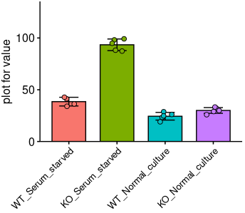
- 基础绘图
plot_basic <- plot_bar_basic(test_data, x = "group", y = "value", ylab = "plot for value")
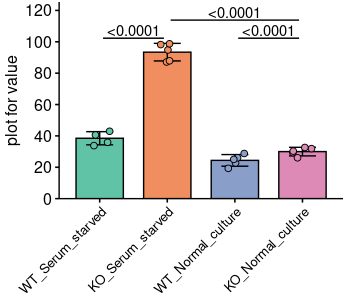
- 根据参数进一步标记显著性,仅作参考,你也可以适当的手动调整
plot_stat <- plot_basic +
  scale_fill_manual(
    values = c("#60c3a6", "#f18e5f", "#8a9eca", "#de8ab7")
  ) +
  scale_y_continuous(breaks = seq(0, 160, by = 20), expand = c(0,0), limits = c(0,plot_para$y_lim)) +
  # WT_Serum_starved vs. KO_Serum_starved
  annotate("segment", x = 1.05, xend = 1.95, y = plot_para[[2]])+
  annotate("text", x = 1.5, y = plot_para[[2]] + plot_para[[3]]*1.5, label = plot_para[[1]]["WT_Serum_starved-KO_Serum_starved"])+
  # WT_Normal_culture vs. KO_Serum_starved
  annotate("segment", x = 3.05, xend = 3.95, y = plot_para[[2]])+
  annotate("text", x = 3.5, y = plot_para[[2]] + plot_para[[3]]*1.5, label = plot_para[[1]]["WT_Normal_culture-KO_Serum_starved"])+
  # KO_Serum_starved vs. KO_Normal_culture
  annotate("segment", x = 2.05, xend = 3.95, y = plot_para[[2]]+ plot_para[[3]]*3.5)+
  annotate("text", x = 3, y = plot_para[[2]] + plot_para[[3]]*5, label = plot_para[[1]]["KO_Serum_starved-KO_Normal_culture"])
plot_stat
对于两组来说,就不需要get_plot_para这个函数了,我们plot_bar_basic基础上在简单编辑可以。
这里提供脚本封装内的函数p_to_star的使用示例,可以把p值转换为星号。
filter_basic <- plot_bar_basic(test_data_filter, x = "group", y = "value", ylab = "plot for value")

# 转换为星号(单个p值转换)
p_label <- p_to_stars(stat_filter_res[[1]]$p.value)
# 如果是多组多个p值,可以是这样使用:
# p_label <- sapply(stat_filter_res[[1]]$p.value, p_to_stars)

filter_stat_plot <- filter_basic +
  scale_fill_manual(
    values = c("#60c3a6", "#00a54f")
  ) +
  scale_y_continuous(breaks = seq(0, 120, by = 20), expand = c(0,0), limits = c(0, 120)) +
  # aov/kw p.value
  annotate("segment", x = 1, xend = 2, y = 110) +
  annotate("text", x = 1.5, y = 112, label = p_label, size = 8)

filter_stat_plot

10. 场景应用:基于多分组bulk转录组对基因进行表达量统计分析(仅作展示,不提供数据)
现在有一个多分组的bulk转录组数据,以及对应的meta信息。看看如何应用上述函数,便捷地实现统计。
- 首先查看一下数据
# 这是一个经过DESeq2标准化后地矩阵
exprSet_vst[1:4,1:4]
#             W81      W83      W84      W80
# Lyz2   18.57773 18.81743 18.98225 18.92183
# Mt-co1 18.29783 18.89893 18.64288 18.55819
# Sftpc  17.59295 18.24031 18.13995 18.04844
# Mt-co3 16.58128 17.23893 17.41379 17.52487

# 对应地meta信息
head(datTraits)
#     sample group sample2     RVSP    Fulton     RVID  PAT.PET    TAPSE        CO group2
# W81    W81   CON  Cont_2  32.4500 0.2647000 1.678753 0.450777 2.389750 114.04988    CON
# W83    W83   CON  Cont_3  29.3237 0.2593000 1.530280 0.305483 2.518139  92.83599    CON
# W84    W84   CON  Cont_4  31.9598 0.2881500 1.357813 0.345269 2.241625  68.61000    CON
# W80    W80   CON  Cont_1  30.8033 0.2437100 1.589875 0.287154 2.103375  73.24000    CON
# A84    A84  SuHx  SuHx_6 106.6120 0.6791720 2.567500 0.132184 2.537875  44.53881   SuHx
# A96    A96  SuHx  SuHx_1 119.5660 0.8120392 2.853875 0.183333 2.024375  76.80200   SuHx
- 对数据进行整理,并提取拟统计的目标基因
# 添加干预因素的信息
datTraits$suhx <- ifelse(datTraits$group == "CON", "con", "suhx")
datTraits$inulin <- ifelse(datTraits$group %in% c("CON", "SuHx"), "con", "inulin")
datTraits$gw <- ifelse(datTraits$group == "SuHx-IN+GW", "gw", "con")

# 提取基因信息表达量信息
datExpr2 <- t(exprSet_vst)
gene_to_use = c("Fanci", "Fancd2", "H2ax", "Fancl")
gene_to_use = gene_to_use[gene_to_use %in% colnames(datExpr2)]

# 合并,只保留有用信息
data <- cbind(datTraits, datExpr2[,gene_to_use]) %>%
  select(all_of(c("sample", "group", "RVSP", "Fulton", "RVID", "PAT.PET",
                  "TAPSE", "CO", "inulin", "suhx", "gw", "Fanci", "Fancd2",
                  "H2ax", "Fancl")))

head(data)
#     sample group     RVSP    Fulton     RVID  PAT.PET    TAPSE        CO inulin suhx  gw    Fanci   Fancd2     H2ax    Fancl
# W81    W81   CON  32.4500 0.2647000 1.678753 0.450777 2.389750 114.04988    con  con con 6.479441 6.544456 8.813432 7.686432
# W83    W83   CON  29.3237 0.2593000 1.530280 0.305483 2.518139  92.83599    con  con con 6.713148 6.379477 8.215798 7.830406
# W84    W84   CON  31.9598 0.2881500 1.357813 0.345269 2.241625  68.61000    con  con con 6.782347 6.746125 8.837235 7.967137
# W80    W80   CON  30.8033 0.2437100 1.589875 0.287154 2.103375  73.24000    con  con con 6.610660 6.390644 8.596658 7.927415
# A84    A84  SuHx 106.6120 0.6791720 2.567500 0.132184 2.537875  44.53881    con suhx con 6.902632 6.851762 8.928339 7.597125
# A96    A96  SuHx 119.5660 0.8120392 2.853875 0.183333 2.024375  76.80200    con suhx con 6.621814 6.605791 8.838876 7.687908
- 接下来我们写一个临时函数,把三个函数都封装进去
# 批量进行统计学分析
stat_fc <- function(data, gene){
  nor <- test_assumptions(data, gene, "group")
  stat <- auto_stat_test(data, nor, gene, "group", factors = c("suhx", "inulin", "gw"))
  stat_summary <- stat_res_collect(data, nor, stat, glue::glue("Fig6_{gene}"))

  return(stat_summary)
}
- 执行
stats_res_list <- lapply(gene_to_use, function(i) stat_fc(data = data, gene = i))
names(stats_res_list) <- gene_to_use

最终获取的结果,就是一个基因对应一个list,结构如前所述。list第一个结构是纳入分析的数据,即这里的data;第二个结构是统计的汇总数据框,如下:
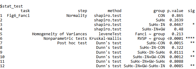
最后只需要循环保存就行
for (g in gene_to_use) {
  res_use <- stats_res_list[[g]]
  openxlsx::write.xlsx(res_use, file = glue::glue("results/{g}_stat_res.xlsx"))
}

 浙公网安备 33010602011771号