逻辑回归实例

　　简介

　　Logistic回归是一种机器学习分类算法，用于预测分类因变量的概率。在逻辑回归中，因变量是一个二进制变量，包含编码为1（是，成功等）或0（不，失败等）的数据。换句话说，逻辑回归模型预测P（Y = 1）是X的函数。

　　数据

　　该数据集来自UCI机器学习库，它与葡萄牙银行机构的直接营销活动（电话）有关。分类目标是预测客户是否将购买定期存款（变量y）。数据集可以从这里下载或者here。

import pandas as pd
import numpy as np
from sklearn import preprocessing
import matplotlib.pyplot as plt 
plt.rc("font", size=14)
from sklearn.linear_model import LogisticRegression
from sklearn.cross_validation import train_test_split
import seaborn as sns
sns.set(style="white")
sns.set(style="whitegrid", color_codes=True)

data=pd.read_csv('F:/wd.jupyter/datasets/log_data/bank.csv',delimiter=';')
data=data.dropna()
print(data.shape)
print(list(data.columns))

data.head()

(41188, 21)
['age', 'job', 'marital', 'education', 'default', 'housing', 'loan', 'contact', 'month', 'day_of_week', 'duration', 'campaign', 'pdays', 'previous', 'poutcome', 'emp.var.rate', 'cons.price.idx', 'cons.conf.idx', 'euribor3m', 'nr.employed', 'y']

　　数据集提供银行客户的信息。它包括41,188条记录和21个字段。

　　变量

age (numeric)
job : type of job (categorical: “admin”, “blue-collar”, “entrepreneur”, “housemaid”, “management”, “retired”, “self-employed”, “services”, “student”, “technician”, “unemployed”, “unknown”)
marital : marital status (categorical: “divorced”, “married”, “single”, “unknown”)
education (categorical: “basic.4y”, “basic.6y”, “basic.9y”, “high.school”, “illiterate”, “professional.course”, “university.degree”, “unknown”)
default: has credit in default? (categorical: “no”, “yes”, “unknown”)
housing: has housing loan? (categorical: “no”, “yes”, “unknown”)
loan: has personal loan? (categorical: “no”, “yes”, “unknown”)
contact: contact communication type (categorical: “cellular”, “telephone”)
month: last contact month of year (categorical: “jan”, “feb”, “mar”, …, “nov”, “dec”)
day_of_week: last contact day of the week (categorical: “mon”, “tue”, “wed”, “thu”, “fri”)
duration: last contact duration, in seconds (numeric). Important note: this attribute highly affects the output target (e.g., if duration=0 then y=’no’). The duration is not known before a call is performed, also, after the end of the call, y is obviously known. Thus, this input should only be included for benchmark purposes and should be discarded if the intention is to have a realistic predictive model
campaign: number of contacts performed during this campaign and for this client (numeric, includes last contact)
pdays: number of days that passed by after the client was last contacted from a previous campaign (numeric; 999 means client was not previously contacted)
previous: number of contacts performed before this campaign and for this client (numeric)
poutcome: outcome of the previous marketing campaign (categorical: “failure”, “nonexistent”, “success”)
emp.var.rate: employment variation rate — (numeric)
cons.price.idx: consumer price index — (numeric)
cons.conf.idx: consumer confidence index — (numeric)
euribor3m: euribor 3 month rate — (numeric)
nr.employed: number of employees — (numeric)

　　预测变量

　　y - 客户是否订购了定期存款？（二进制：“1”表示“是”，“0”表示“否”）

　　数据集的教育列有许多类别，我们需要减少类别以获得更好的建模。教育专栏有以下几类：　

data['education'].unique()

array(['basic.4y', 'high.school', 'basic.6y', 'basic.9y',
       'professional.course', 'unknown', 'university.degree',
       'illiterate'], dtype=object)

　　让我们将“basic.4y”，“basic.9y”和“basic.6y”组合在一起，称之为“basic”。　

data['education']=np.where(data['education']=='basic.4y','basic',data['education'])
data['education']=np.where(data['education']=='basic.6y','basic',data['education'])
data['education']=np.where(data['education']=='basic.9y','basic',data['education'])
data['education'].unique()

array(['basic', 'high.school', 'professional.course', 'unknown',
       'university.degree', 'illiterate'], dtype=object)

　　如果不懂np.where函数，可以看这里。

　　数据探索

　　信息总览

data.info()

<class 'pandas.core.frame.DataFrame'>
Int64Index: 41188 entries, 0 to 41187
Data columns (total 21 columns):
age               41188 non-null int64
job               41188 non-null object
marital           41188 non-null object
education         41188 non-null object
default           41188 non-null object
housing           41188 non-null object
loan              41188 non-null object
contact           41188 non-null object
month             41188 non-null object
day_of_week       41188 non-null object
duration          41188 non-null int64
campaign          41188 non-null int64
pdays             41188 non-null int64
previous          41188 non-null int64
poutcome          41188 non-null object
emp.var.rate      41188 non-null float64
cons.price.idx    41188 non-null float64
cons.conf.idx     41188 non-null float64
euribor3m         41188 non-null float64
nr.employed       41188 non-null float64
y                 41188 non-null object
dtypes: float64(5), int64(5), object(11)
memory usage: 6.9+ MB

　　可以看到，有5列float64数据，有5列int64数据，有11列object。

　　把y变为数值型，并进行简单的统计。　

data.loc[data['y']=='yes','y']=1
data.loc[data['y']=='no','y']=0
data['y'].value_counts()

0    36548
1     4640
Name: y, dtype: int64

sns.countplot(x='y',data=data,palette='hls')

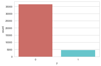
　　因变量中有36548个没有，4640个是。

　　让我们深入了解这两个类别。

data.groupby('y').mean()

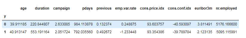
可以看到：

　　购买定期存款的客户的平均年龄高于未购买定期存款的客户的平均年龄。
　　对于购买它的客户来说，pdays（自上次联系客户以来的日子）可以理解的更低。 pdays越低，最后一次通话的记忆越好，因此销售的机会就越大。
　　令人惊讶的是，购买定期存款的客户的广告系列（compaign当前广告系列期间的联系人或通话次数）较低。
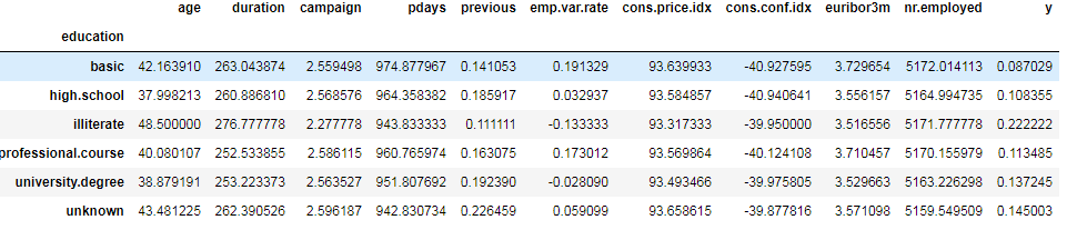
　　我们可以计算其他分类变量（如教育和婚姻状况）的分类方法，以更详细地了解我们的数据。

data.groupby('education').mean()

data.groupby('marital').mean()

　　可视化

　　工作和y的关系

pd.crosstab(data.job,data.y).plot(kind='bar')
plt.title('Purchase Frequency for Job Title')
plt.xlabel('Job')
plt.ylabel('Frequency of Purchase')
#plt.savefig('purchase_fre_job')

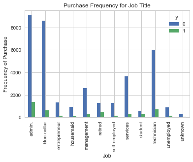
购买存款的频率在很大程度上取决于职位。因此，职称可以是结果变量的良好预测因子。

　　婚姻状况与y的关系：

table=pd.crosstab(data.marital,data.y)
table.div(table.sum(axis=1).astype(float), axis=0).plot(kind='bar', stacked=True)
plt.title('Stacked Bar Chart of Marital Status vs Purchase')
plt.xlabel('Marital Status')
plt.ylabel('Proportion of Customers')

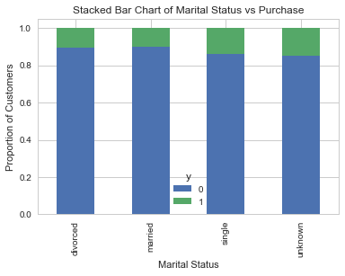
婚姻状况似乎不是结果变量的强预测因子。

　　教育情况与y的关系

table=pd.crosstab(data.education,data.y)
table.div(table.sum(axis=1).astype(float),axis=0).plot(kind='bar')
plt.title('Stacked Bar Chart of Education Status vs Purchase')
plt.xlabel('Education Status')
plt.ylabel('Proportion of Customers')

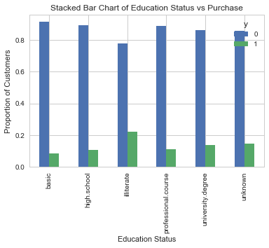
教育似乎是良好预测指标。

　　day_of_week与y的关系：

pd.crosstab(data.day_of_week,data.y).plot(kind='bar')
plt.title('Purchase Frequency for Day of Week')
plt.xlabel('Day of Week')
plt.ylabel('Frequency of Purchase')
plt.savefig('pur_dayofweek_bar')

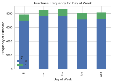
Day of week 或许不是一个良好的预测指标。

　　month与y的关系

pd.crosstab(data.month,data.y).plot(kind='bar')
plt.title('Purchase Frequency for Month')
plt.xlabel('Month')
plt.ylabel('Frequency of Purchase')
plt.savefig('pur_fre_month_bar')

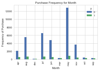
Month是一个良好的预测指标。

　　年龄的分布：

data.age.hist()
plt.title('Histogram of Age')
plt.xlabel('Age')
plt.ylabel('Frequency')

该数据集中银行的大多数客户的年龄范围为30-40。

　　poutcome与y的关系：

pd.crosstab(data.poutcome,data.y).plot(kind='bar')
plt.title('Purchase Frequency for Poutcome')
plt.xlabel('Poutcome')
plt.ylabel('Frequency of Purchase')

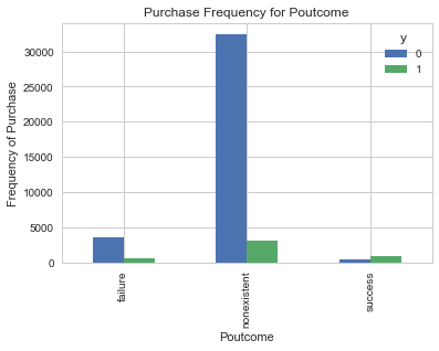
poutcome是一个良好的预测指标。

　　创建虚拟变量

　　这是只有两个值的变量，0和1。

　　回顾我们数据集的信息，有11个object，其中y已经转化过来，另外有10个类别需要转化。

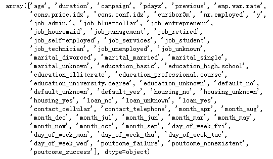
cat_vars=['job','marital','education','default','housing','loan','contact','month','day_of_week','poutcome']
for var in cat_vars:
    cat_list='var'+'_'+var
    cat_list = pd.get_dummies(data[var], prefix=var)
    data1=data.join(cat_list)
    data=data1
    

data_vars=data.columns.values.tolist()
to_keep=[i for i in data_vars if i not in cat_vars]


data_final=data[to_keep]
data_final.columns.values

最终的数据

　　分离特征与目标变量

data_final_vars=data_final.columns.values.tolist()
y=['y']
X=[i for i in data_final_vars if i not in y]

　　 特征选择　

　　递归特征消除（Recursive Feature Elimination，RFE）基于以下思想：首先，在初始特征集上训练估计器，并且通过coef_属性或通过feature_importances_属性获得每个特征的重要性。然后，从当前的一组特征中删除最不重要的特征。在修剪的集合上递归地重复该过程，直到最终到达所需数量的要选择的特征。

from sklearn import datasets
from sklearn.feature_selection import RFE
from sklearn.linear_model import LogisticRegression
logreg = LogisticRegression()
rfe = RFE(logreg, 18)
rfe = rfe.fit(data_final[X], data_final[y] )
print(rfe.support_)
print(rfe.ranking_)

根据布尔值筛选我们想要的特征(参考）：

from itertools import compress

cols=list(compress(X,rfe.support_))
cols

或者：
cols= [i for index,i in list(enumerate(X)) if rfe.support_[index] == True]

　　执行模型

import statsmodels.api as sm

X=data_final[cols]
y=data_final['y']


logit_model=sm.Logit(y,X)
logit_model.raise_on_perfect_prediction = False
result=logit_model.fit()
print(result.summary().as_text)

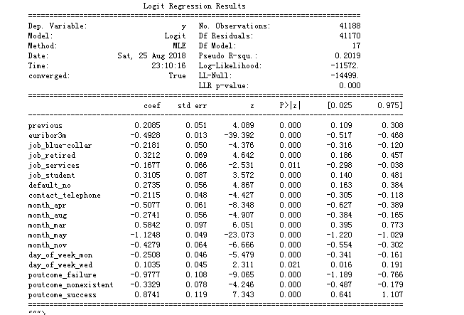
　　大多数变量的p值小于0.05，因此，大多数变量对模型都很重要。

　逻辑回归模型的拟合

from sklearn.linear_model import LogisticRegression
from sklearn import metrics

X_train, X_test, y_train, y_test = train_test_split(X, y, test_size=0.3, random_state=0)
logreg = LogisticRegression()
logreg.fit(X_train, y_train)
y_pred = logreg.predict(X_test)
y_pred = logreg.predict(X_test)
print('Accuracy of logistic regression classifier on test set: {:.2f}'.format(logreg.score(X_test, y_test)))

　　可以看到，准确率达到了0.9.

　　交叉验证

　　交叉验证尝试避免过度拟合，同时仍然为每个观察数据集生成预测。我们使用10折交叉验证来训练我们的Logistic回归模型。

from sklearn import model_selection
from sklearn.model_selection import cross_val_score

kfold = model_selection.KFold(n_splits=10, random_state=7)
modelCV = LogisticRegression()
scoring = 'accuracy'
results = model_selection.cross_val_score(modelCV, X_train, y_train, cv=kfold, scoring=scoring)
print("10-fold cross validation average accuracy: %.3f" % (results.mean()))

平均精度仍然非常接近Logistic回归模型的准确度; 因此，我们可以得出结论，我们的模型很好拟合了数据。

　Confusion Matrix

from sklearn.metrics import confusion_matrix

confusion_matrix = confusion_matrix(y_test, y_pred)
print(confusion_matrix)

结果告诉我们，我们有10848 + 2564个正确预测和1124 + 121个错误预测。

　　计算精度（precision）召回(recall)F测量(F-measure)和支持(support)

精度是比率tp /（tp + fp），其中tp是真阳性的数量，fp是假阳性的数量。精确度直观地是分类器如果是负的则不将样品标记为阳性的能力。

召回是比率tp /（tp + fn）其中tp是真阳性的数量，fn是假阴性的数量。召回直观地是分类器找到所有阳性样本的能力。

F-beta分数可以解释为精确度和召回率的加权调和平均值，其中F-β分数在1处达到其最佳值，在0处达到最差分数。

F-beta评分对召回的重量超过精确度β因子。 beta = 1.0意味着召回和精确度同样重要。

支持是y_test中每个类的出现次数。

from sklearn.metrics import classification_report

print(classification_report(y_test, y_pred))

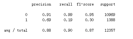
可以看出：在整个测试集中，88％的促销定期存款是客户喜欢的定期存款。在整个测试集中，90％的客户首选定期存款。

　　Macro F1 Score

from sklearn.metrics import f1_score

print(f1_score(y_test, y_pred, average = 'macro'))

0.6217653450907061

　　ROC曲线

from sklearn.metrics import roc_auc_score
from sklearn.metrics import roc_curve

logit_roc_auc = roc_auc_score(y_test, logreg.predict(X_test))
fpr, tpr, thresholds = roc_curve(y_test, logreg.predict_proba(X_test)[:,1])
plt.figure()
plt.plot(fpr, tpr, label='Logistic Regression (area = %0.2f)' % logit_roc_auc)
plt.plot([0, 1], [0, 1],'r--')
plt.xlim([0.0, 1.0])
plt.ylim([0.0, 1.05])
plt.xlabel('False Positive Rate')
plt.ylabel('True Positive Rate')
plt.title('Receiver operating characteristic')
plt.legend(loc="lower right")
#plt.savefig('Log_ROC')
plt.show()

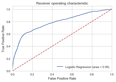
　　ROC曲线是与二元分类器一起使用的另一种常用工具。虚线表示纯随机分类器的ROC曲线; 一个好的分类器尽可能远离该线（朝左上角）。

posted @ 2018-08-25 23:53 Jin_liang 阅读(16914) 评论(0) 编辑收藏举报

会员力量，点亮园子希望

刷新页面返回顶部

Jin_liang

逻辑回归实例

数据

变量

预测变量

数据探索

可视化

创建虚拟变量

执行模型

逻辑回归模型的拟合

交叉验证

Confusion Matrix

计算精度（precision）召回(recall)F测量(F-measure)和支持(support)

ROC曲线

公告

　　数据

　　变量

　　预测变量

　　数据探索

　　可视化

　　创建虚拟变量

　　执行模型

　逻辑回归模型的拟合

　　交叉验证

　Confusion Matrix

　　计算精度（precision）召回(recall)F测量(F-measure)和支持(support)

　　ROC曲线