第一次作业:深度学习基础
1. 视频学习心得及问题总结
1.1绪论
“人工智能”的概念诞生于1956年的达特茅斯会议。

2018年Yoshua Bengio、Geoffrey Hinton、Yann LeCun因在人工智能深度学习方面的贡献获得图灵奖。
人工智能的发展阶段:萌芽期、启动期、消沉期、突破期、发展期、高速发展期。
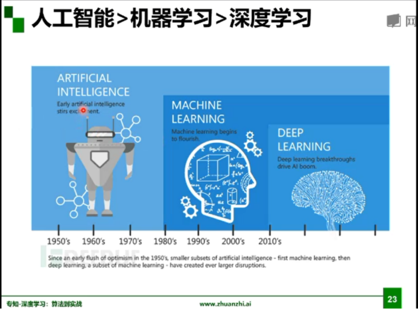
人工智能、机器学习以及深度学习三者之间的关系:
人工智能是一个领域,就是一个目标,我们希望机器人像人一样的去感知、去思考,机器学习的是来实现这样一个目标的,而深度学习是其中很小的一个点。
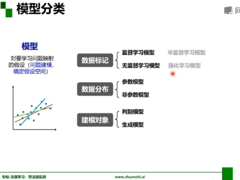
模型分类:
从数据标记角度分类为监督学习、无监督学习、半监督学习、强化学习;
从数据分布角度分类为参数模型、非参数模型;
从建模对象角度分类为判别模型、生成模型;
传统机器学习与深度学习:
前深度学习时代,首先花几天时间收集并标注图像,然后花几个月观察图像,设计一些特征,最后使用某种分类器进行分类;
深度学习时代,首先花几个星期收集并标注图像,然后挑几个深度模型,选几组模型超参数,最后让机器优化模型;


发展历程:
(1)感知器出现,认为感知器无所不能,但是实际上无法解决异或门问题;
(2)BP算法:Rumelhart和Hinton合作在Nature杂志上发表论文,第一次简洁地阐述了
BP算法,在神经网络里增加一个所谓的隐层,解决了XOR难题;
(3)CNN网络:Yann Lecun在1989年发表了论文,之后又进一步运用了一种叫做卷积神经网络的技术,最开始是运用于银行对数字的识别;
(4)Vladmir Vapnik提出了SVM,把神经网络推向寒冬;
(5)Hinton拿到资金后,将神经网络更名为深度学习;
(6)吴恩达2009年发表了论文,解决了速度问题,使用GPU运行速度和用传统双核CPU相比,最快时要快近70倍;
(7)李菲菲建立第一个超大型图像数据库供计算机视觉研究者使用;
(8)Hinton和两个研究生利用CNN+Dropout+Relu激励函数将ILSVRC的错误率降到了15.3%,是人工智能技术突破的一个转折点;
(9)Yoshua Bengio在2011年发表论文,提出了一种修正的relu激励函数,解决了传统激励函数在反向传播计算中的梯度消失问题;
(10)Schmidhuber和他的学生提出来长短期记忆的计算模型。
1.2深度学习概述
深度学习有六大不能:
(1)稳定性低;(2)可调试性差;(3)参数不透明;(4)机器偏见;(5)增量性差;(6)推理能力差;

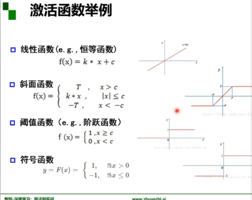
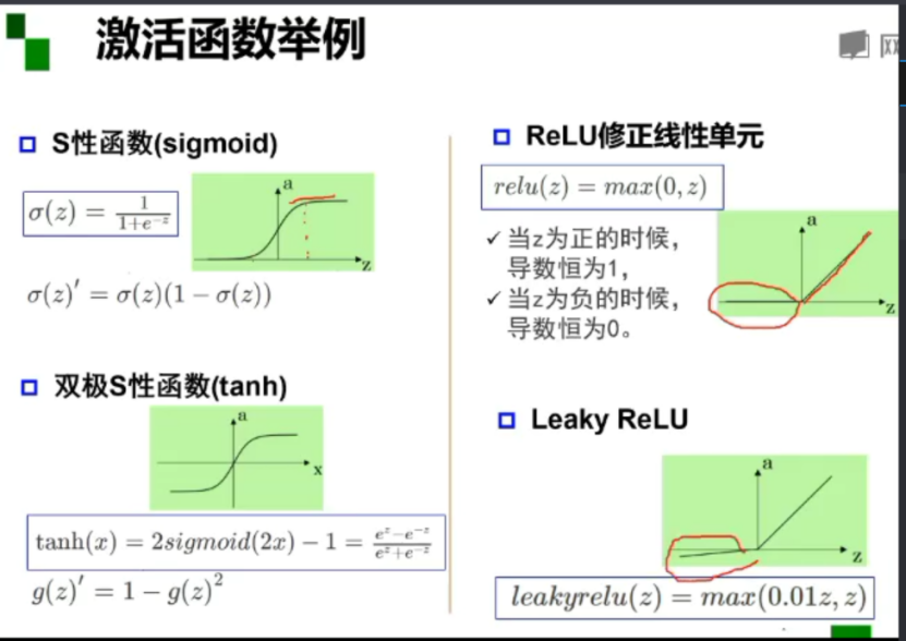
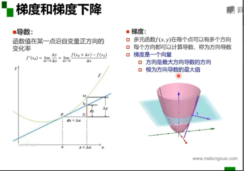
激活函数:激活函数是用来加入非线性因素的,提高神经网络对模型的表达能力,解决线性模型所不能解决的问题。假设一个示例神经网络中仅包含线性卷积和全连接运算,那么该网络仅能够表达线性映射,即便增加网络的深度也依旧还是线性映射,难以有效建模实际环境中非线性分布的数据。
梯度:是一个向量,方向是最大方向导数的方向,模为方向导数的最大值。
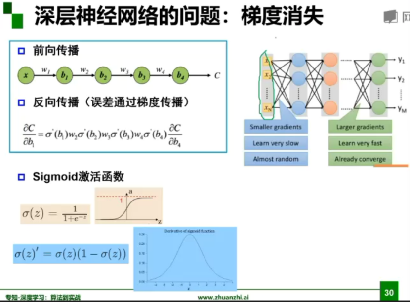
深层神经网络的问题:梯度消失
对于激活函数,之前一直使用Sigmoid函数,其函数图像成一个S型,它会将正无穷到负无穷的数映射到0~1之间。当我们对Sigmoid函数求导时,会呈现一个驼峰状(很像高斯函数),从求导结果可以看出,Sigmoid导数的取值范围在0~0.25之间,而我们初始化的网络权值通常都小于1,因此,当层数增多时,小于0的值不断相乘,最后就导致梯度消失的情况出现。
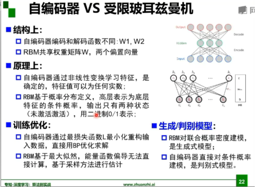
受限玻尔兹曼机和自编码器:
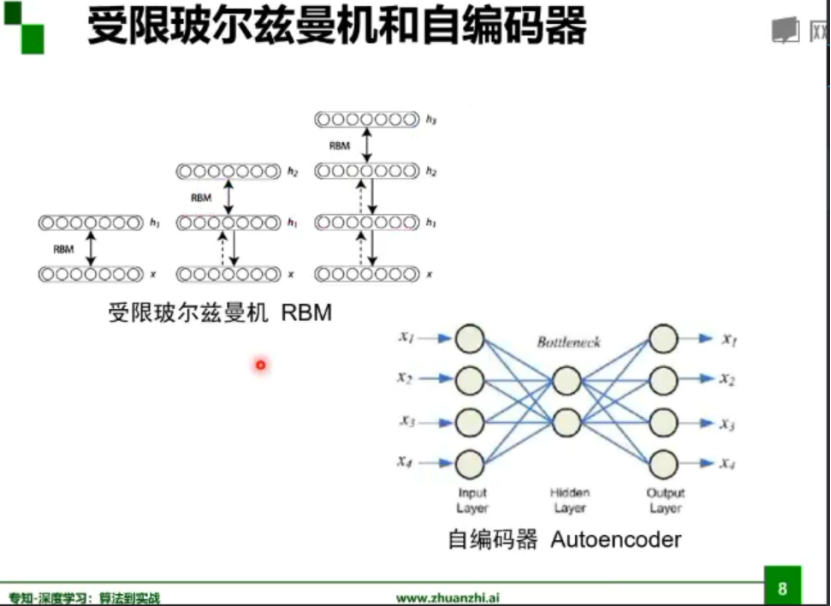
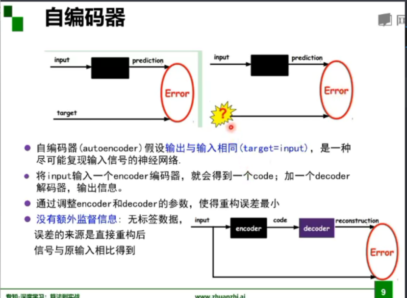
自编码器:
2. 代码练习
2.1图像处理基本练习
!wget https://raw.githubusercontent.com/summitgao/ImageGallery/master/yeast_colony_array.jpg
import matplotlib
import numpy as np
import matplotlib.pyplot as plt

import skimage
from skimage import data
from skimage import io

colony = io.imread('yeast_colony_array.jpg')
print(type(colony))
print(colony.shape)
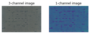
# Plot all channels of a real image
plt.subplot(121)
plt.imshow(colony[:,:,:])
plt.title('3-channel image')
plt.axis('off')

# Plot one channel only
plt.subplot(122)
plt.imshow(colony[:,:,0])
plt.title('1-channel image')
plt.axis('off');
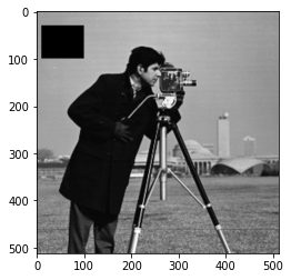
# Get the pixel value at row 10, column 10 on the 10th row and 20th column
camera = data.camera()
print(camera[10, 20])

# Set a region to black
camera[30:100, 10:100] = 0
plt.imshow(camera, 'gray')
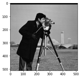
# Set the first ten lines to black
camera = data.camera()
camera[:10] = 0
plt.imshow(camera, 'gray')
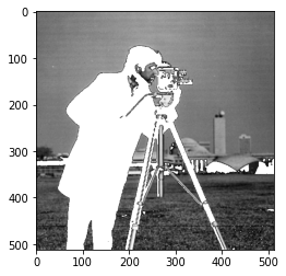
# Set to "white" (255) pixels where mask is True
camera = data.camera()
mask = camera < 80
camera[mask] = 255
plt.imshow(camera, 'gray')
# Change the color for real images
cat = data.chelsea()
plt.imshow(cat)

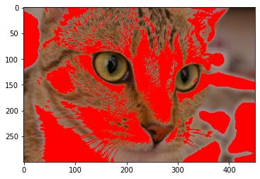
# Set brighter pixels to red
red_cat = cat.copy()
reddish = cat[:, :, 0] > 160
red_cat[reddish] = [255, 0, 0]
plt.imshow(red_cat)
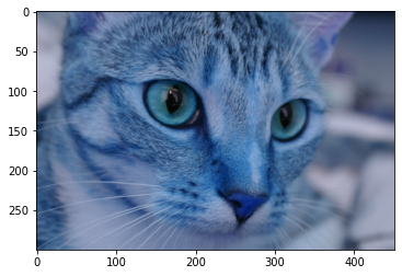
# Change RGB color to BGR for openCV
BGR_cat = cat[:, :, ::-1]
plt.imshow(BGR_cat)
from skimage import img_as_float, img_as_ubyte
float_cat = img_as_float(cat)
uint_cat = img_as_ubyte(float_cat)
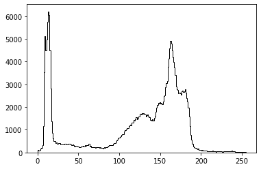
img = data.camera()
plt.hist(img.ravel(), bins=256, histtype='step', color='black');
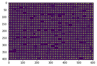
# Use colony image for segmentation
colony = io.imread('yeast_colony_array.jpg')
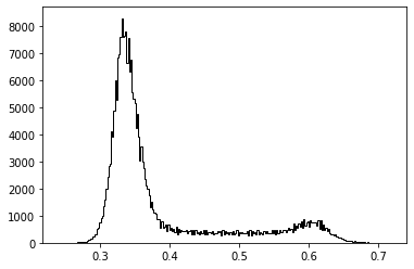
# Plot histogram
img = skimage.color.rgb2gray(colony)
plt.hist(img.ravel(), bins=256, histtype='step', color='black');
# Use thresholding
plt.imshow(img>0.5)
from skimage.feature import canny
from scipy import ndimage as ndi
img_edges = canny(img)
img_filled = ndi.binary_fill_holes(img_edges)

# Plot
plt.figure(figsize=(18, 12))
plt.subplot(121)
plt.imshow(img_edges, 'gray')
plt.subplot(122)
plt.imshow(img_filled, 'gray')

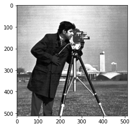
# Load an example image
img = data.camera()
plt.imshow(img, 'gray')
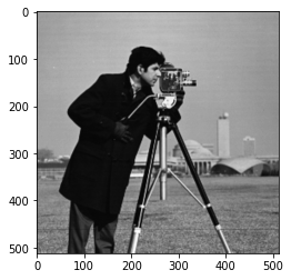
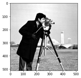
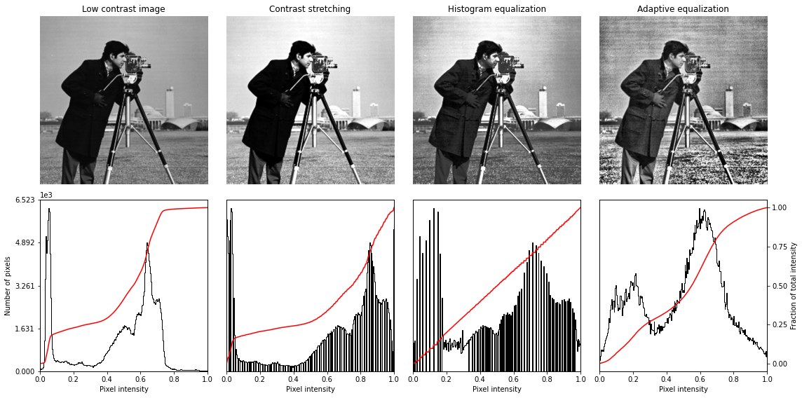
from skimage import exposure
# Contrast stretching
p2, p98 = np.percentile(img, (2, 98))
img_rescale = exposure.rescale_intensity(img, in_range=(p2, p98))
plt.imshow(img_rescale, 'gray')
# Equalization
img_eq = exposure.equalize_hist(img)
plt.imshow(img_eq, 'gray')
# Adaptive Equalization
img_adapteq = exposure.equalize_adapthist(img, clip_limit=0.03)
plt.imshow(img_adapteq, 'gray')
# Display results
def plot_img_and_hist(img, axes, bins=256):
    """Plot an image along with its histogram and cumulative histogram.

    """
    img = img_as_float(img)
    ax_img, ax_hist = axes
    ax_cdf = ax_hist.twinx()

    # Display image
    ax_img.imshow(img, cmap=plt.cm.gray)
    ax_img.set_axis_off()
    ax_img.set_adjustable('box')

    # Display histogram
    ax_hist.hist(img.ravel(), bins=bins, histtype='step', color='black')
    ax_hist.ticklabel_format(axis='y', style='scientific', scilimits=(0, 0))
    ax_hist.set_xlabel('Pixel intensity')
    ax_hist.set_xlim(0, 1)
    ax_hist.set_yticks([])

    # Display cumulative distribution
    img_cdf, bins = exposure.cumulative_distribution(img, bins)
    ax_cdf.plot(bins, img_cdf, 'r')
    ax_cdf.set_yticks([])

    return ax_img, ax_hist, ax_cdf
fig = plt.figure(figsize=(16, 8))
axes = np.zeros((2, 4), dtype=np.object)
axes[0, 0] = fig.add_subplot(2, 4, 1)
for i in range(1, 4):
    axes[0, i] = fig.add_subplot(2, 4, 1+i, sharex=axes[0,0], sharey=axes[0,0])
for i in range(0, 4):
    axes[1, i] = fig.add_subplot(2, 4, 5+i)

ax_img, ax_hist, ax_cdf = plot_img_and_hist(img, axes[:, 0])
ax_img.set_title('Low contrast image')

y_min, y_max = ax_hist.get_ylim()
ax_hist.set_ylabel('Number of pixels')
ax_hist.set_yticks(np.linspace(0, y_max, 5))

ax_img, ax_hist, ax_cdf = plot_img_and_hist(img_rescale, axes[:, 1])
ax_img.set_title('Contrast stretching')

ax_img, ax_hist, ax_cdf = plot_img_and_hist(img_eq, axes[:, 2])
ax_img.set_title('Histogram equalization')

ax_img, ax_hist, ax_cdf = plot_img_and_hist(img_adapteq, axes[:, 3])
ax_img.set_title('Adaptive equalization')

ax_cdf.set_ylabel('Fraction of total intensity')
ax_cdf.set_yticks(np.linspace(0, 1, 5))

fig.tight_layout()
plt.show()
2.2 pytorch基础练习
#一个数
import torch
x = torch.tensor(125)
print(x)
#一维数组
x = torch.tensor([1,2,3])
print(x)

#二维数组
x = torch.ones(2,3)
print(x)

#任意维数组
x = torch.ones(3,3,3)
print(x)

#创建空张量
x = torch.empty(3,3)
print(x)

#创建一个随机初始化的张量
x = torch.rand(3,3)
print(x)

#创建一个全为0的张量,并将数据类型设为long
x = torch.zeros(3,3,dtype=torch.long)
print(x)

#基于现有的tensor,创建一个新的tensor,使新的tensor可以继承原有tensor的属性
y = x.new_ones(3,3)
print(y)

#继承原来tensor的大小,重新定义了数据类型
z = torch.randn_like(x,dtype = torch.float)
print(z)
tensor([1, 2, 3])
tensor([[1., 1., 1.],
        [1., 1., 1.]])
tensor([[[1., 1., 1.],
         [1., 1., 1.],
         [1., 1., 1.]],

        [[1., 1., 1.],
         [1., 1., 1.],
         [1., 1., 1.]],

        [[1., 1., 1.],
         [1., 1., 1.],
         [1., 1., 1.]]])
tensor([[1.6773e-35, 0.0000e+00, 3.3631e-44],
        [0.0000e+00,        nan, 0.0000e+00],
        [1.1578e+27, 1.1362e+30, 7.1547e+22]])
tensor([[0.2663, 0.1039, 0.7578],
        [0.3250, 0.3323, 0.2042],
        [0.7675, 0.9358, 0.9857]])
tensor([[0, 0, 0],
        [0, 0, 0],
        [0, 0, 0]])
tensor([[1, 1, 1],
        [1, 1, 1],
        [1, 1, 1]])
tensor([[ 1.2492,  1.5812,  1.3829],
        [-0.9308, -0.6413,  0.7611],
        [-0.8240, -0.1809, -1.6046]])
#创建一个2x4的tensor,用Tensor创建出来的是浮点数,用tensor创建出来的是长整型
m = torch.tensor([[2,5,3,7],[4,2,1,9]])
print(m.size(0),m.size(1),m.size(),sep = '-')

#返回m中元素的数量
print(m.numel())

#返回m中的元素,利用下标标记元素
print(m[0][2])
print(m[:,1])
print(m[0,:])

#点乘
v = torch.arange(1, 5)
m @ v
m[[0], :] @ v

#加法
m + torch.rand(2, 4)

#转置
print(m.t())
print(m.transpose(0,1))

#返回3到8之间等距的20个数
torch.linspace(3,8,20)

#转换数据类型并显示
from matplotlib import pyplot as plt
plt.hist(torch.randn(1000).numpy(),100);
2-4-torch.Size([2, 4])
8
tensor(3)
tensor([5, 2])
tensor([2, 5, 3, 7])
tensor([[2, 4],
        [5, 2],
        [3, 1],
        [7, 9]])
tensor([[2, 4],
        [5, 2],
        [3, 1],
        [7, 9]])
#数组拼接
a = torch.Tensor([[1,2,3,4]])
b = torch.Tensor([[5,6,7,8]])
print(torch.cat((a,b),0))#在0方向即在Y方向上拼接
print(torch.cat((a,b),1))#在1方向即在X方向上拼接
tensor([[1., 2., 3., 4.],
        [5., 6., 7., 8.]])
tensor([[1., 2., 3., 4., 5., 6., 7., 8.]])
2.3 螺旋数据分类
!wget https://raw.githubusercontent.com/Atcold/pytorch-Deep-Learning/master/res/plot_lib.py
#数据初始化
import random
import torch
from torch import nn, optim
import math
from IPython import display
from plot_lib import plot_data, plot_model, set_default


# 因为colab是支持GPU的,torch 将在 GPU 上运行
device = torch.device("cuda:0" if torch.cuda.is_available() else "cpu")

# 初始化随机数种子。神经网络的参数都是随机初始化的,
# 不同的初始化参数往往会导致不同的结果,当得到比较好的结果时我们通常希望这个结果是可以复现的,
# 因此,在pytorch中,通过设置随机数种子也可以达到这个目的
seed = 12345
random.seed(seed)
torch.manual_seed(seed)

N = 1000  # 每类样本的数量
D = 2  # 每个样本的特征维度
C = 3  # 样本的类别
H = 100  # 神经网络里隐层单元的数量
X = torch.zeros(N * C, D).to(device)
Y = torch.zeros(N * C, dtype=torch.long).to(device)
for c in range(C):
    index = 0
    t = torch.linspace(0, 1, N) # 在[0,1]间均匀的取10000个数,赋给t
    # 下面的代码不用理解太多,总之是根据公式计算出三类样本(可以构成螺旋形)
    # torch.randn(N) 是得到 N 个均值为0,方差为 1 的一组随机数,注意要和 rand 区分开
    inner_var = torch.linspace( (2*math.pi/C)*c, (2*math.pi/C)*(2+c), N) + torch.randn(N) * 0.2

    # 每个样本的(x,y)坐标都保存在 X 里
    # Y 里存储的是样本的类别,分别为 [0, 1, 2]
    for ix in range(N * c, N * (c + 1)):
        X[ix] = t[index] * torch.FloatTensor((math.sin(inner_var[index]), math.cos(inner_var[index])))
        Y[ix] = c
        index += 1
plot_data(X, Y)

#创建线性模型
learning_rate = 1e-3
lambda_l2 = 1e-5

# nn 包用来创建线性模型
# 每一个线性模型都包含 weight 和 bias
model = nn.Sequential(
    nn.Linear(D, H),
    nn.Linear(H, C)
)
model.to(device) # 把模型放到GPU上

# nn 包含多种不同的损失函数,这里使用的是交叉熵(cross entropy loss)损失函数
criterion = torch.nn.CrossEntropyLoss()

# 这里使用 optim 包进行随机梯度下降(stochastic gradient descent)优化
optimizer = torch.optim.SGD(model.parameters(), lr=learning_rate, weight_decay=lambda_l2)

# 开始训练
for t in range(1000):
    # 把数据输入模型,得到预测结果
    y_pred = model(X)
    # 计算损失和准确率
    loss = criterion(y_pred, Y)
    score, predicted = torch.max(y_pred, 1)
    acc = (Y == predicted).sum().float() / len(Y)
    print('[EPOCH]: %i, [LOSS]: %.6f, [ACCURACY]: %.3f' % (t, loss.item(), acc))
    display.clear_output(wait=True)

    # 反向传播前把梯度置 0
    optimizer.zero_grad()
    # 反向传播优化
    loss.backward()
    # 更新全部参数
    optimizer.step()
#效果图如下
# Plot trained model
print(model)
plot_model(X, Y, model)


####当尝试使用线性的决策边界来分隔螺旋的数据 - 只使用nn.linear()模组,而不在之间加上非线性 - 我们只能达到 50% 的正确度。
#加入ReLU激活函数
learning_rate = 1e-3
lambda_l2 = 1e-5
# 这里可以看到,和上面模型不同的是,在两层之间加入了一个 ReLU 激活函数
model = nn.Sequential(
nn.Linear(D, H),
nn.ReLU(),
nn.Linear(H, C)
)
model.to(device)
# 下面的代码和之前是完全一样的,这里不过多叙述
criterion = torch.nn.CrossEntropyLoss()
optimizer = torch.optim.Adam(model.parameters(), lr=learning_rate, weight_decay=lambda_l2) # built-in L2
# 训练模型,和之前的代码是完全一样的
for t in range(1000):
y_pred = model(X)
loss = criterion(y_pred, Y)
score, predicted = torch.max(y_pred, 1)
acc = ((Y == predicted).sum().float() / len(Y))
print("[EPOCH]: %i, [LOSS]: %.6f, [ACCURACY]: %.3f" % (t, loss.item(), acc))
display.clear_output(wait=True)
# zero the gradients before running the backward pass.
optimizer.zero_grad()
# Backward pass to compute the gradient
loss.backward()
# Update params
optimizer.step()
#效果图如下
# Plot trained model
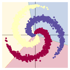
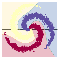
print(model)
plot_model(X, Y, model)
####当我们从线性模型换成在两个 nn.linear() 模组再经过一个 nn.ReLU() 的模型,正确度增加到了 95%。这是因为边界变成非线性的并且更好的顺应资料的螺旋,如下图所呈现的。
2.4 回归分析
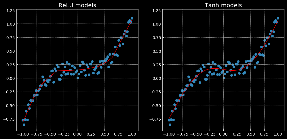
以上表现了一个无法用线性回归完成,但可以用这个相同的网络解决的问题。左面使用了Relu函数,有图使用了tanh函数,前者是一个分段的线性函数,后者则是连续、平滑的回归。

 浙公网安备 33010602011771号