第二次作业：卷积神经网络 part 3

代码练习：

• 完善HybridSN高光谱分类网络

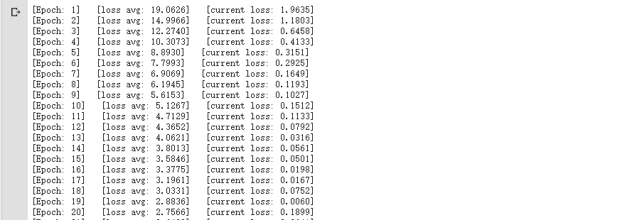
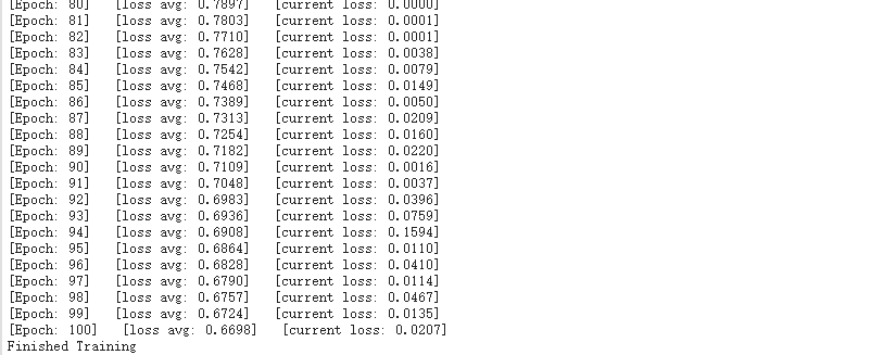
  class HybridSN(nn.Module):
      def __init__(self, stride=1):
          super(HybridSN,self).__init__()
          
          #conv1：（1, 30, 25, 25）， 8个 7x3x3 的卷积核 ==>（8, 24, 23, 23）
          self.conv1 = nn.Conv3d(1, 8, kernel_size=(7,3,3), stride=stride, padding=0)
          self.bn1 = nn.BatchNorm3d(8)#添加BN层
  
          #conv2：（8, 24, 23, 23）， 16个 5x3x3 的卷积核 ==>（16, 20, 21, 21）
          self.conv2 = nn.Conv3d(8, 16, kernel_size=(5,3,3), stride=stride, padding=0)
          self.bn2 = nn.BatchNorm3d(16)
  
          #conv3：（16, 20, 21, 21），32个 3x3x3 的卷积核 ==>（32, 18, 19, 19）
          self.conv3 = nn.Conv3d(16, 32, kernel_size=(3,3,3), stride=stride, padding=0)
          self.bn3 = nn.BatchNorm3d(32)
  
          #二维卷积：（576, 19, 19） 64个 3x3 的卷积核，得到 （64, 17, 17）
          self.conv4 = nn.Conv2d(576, 64, kernel_size=(3,3), stride=stride, padding=0)
          self.bn4 = nn.BatchNorm2d(64)
  
          #接下来是一个 flatten 操作，变为 18496 维的向量，
  		#接下来依次为256，128节点的全连接层，都使用比例为0.4的 Dropout，
  		#最后输出为 16 个节点，是最终的分类类别数
          self.fn1 = nn.Linear(18496,256)
          self.fn2 = nn.Linear(256,128)
          self.fn3 = nn.Linear(128,16)
          self.drop = nn.Dropout(0.4)
           
      def forward(self, x):
        
        out = F.relu(self.bn1(self.conv1(x)))
        out = F.relu(self.bn2(self.conv2(out)))
        out = F.relu(self.bn3(self.conv3(out)))
  
        out = out.reshape(out.shape[0],-1,19,19)
        out = F.relu(self.bn4(self.conv4(out)))  
  
        out = out.reshape(out.shape[0],-1)
          
        out = F.relu(self.drop(self.fn1(out)))
        out = F.relu(self.drop(self.fn2(out)))
        out = self.fn3(out)
        return out
  

  模型训练：

    accuracy                         0.9721      9225
   macro avg     0.9633    0.9256    0.9394      9225
weighted avg     0.9727    0.9721    0.9720      9225

准确率稳定在97.2%左右

修改dropout为0.1，进行测试网络性能和准确率，并在实例化的模型训练之前加入model.train()，在模型测试之前加入model.eval()防止过拟合。

    accuracy                         0.9875      9225
   macro avg     0.9858    0.9844    0.9847      9225
weighted avg     0.9877    0.9875    0.9875      9225

准确率提高到98.6%左右

• SENet实现

  class_num = 16
  
  class SENet(nn.Module):
  
      def __init__(self, planes ,size):
          super(SENet, self).__init__()
  
          self.globalAvgPool = nn.AvgPool2d(size,stride=1)
          self.fc1 = nn.Linear(planes, round(planes / 16))
          self.fc2 = nn.Linear(round(planes / 16), planes)
  
      def forward(self, x):
  
          out = self.globalAvgPool(x)
          out = out.view(out.shape[0], out.shape[1])
          out = F.relu(self.fc1(out))
          out = torch.sigmoid(self.fc2(out))
          
          out = out.view(x.shape[0], x.shape[1], 1, 1)
          out = x * out
          return out
  
  class HybridSN(nn.Module):
      def __init__(self, stride=1):
          super(HybridSN,self).__init__()
          
          #conv1：（1, 30, 25, 25）， 8个 7x3x3 的卷积核 ==>（8, 24, 23, 23）
          self.conv1 = nn.Conv3d(1, 8, kernel_size=(7,3,3), stride=stride, padding=0)
          self.bn1 = nn.BatchNorm3d(8)
          #添加BN层
  
          #conv2：（8, 24, 23, 23）， 16个 5x3x3 的卷积核 ==>（16, 20, 21, 21）
          self.conv2 = nn.Conv3d(8, 16, kernel_size=(5,3,3), stride=stride, padding=0)
          self.bn2 = nn.BatchNorm3d(16)
  
          #conv3：（16, 20, 21, 21），32个 3x3x3 的卷积核 ==>（32, 18, 19, 19）
          self.conv3 = nn.Conv3d(16, 32, kernel_size=(3,3,3), stride=stride, padding=0)
          self.bn3 = nn.BatchNorm3d(32)
  
          #二维卷积：（576, 19, 19） 64个 3x3 的卷积核，得到 （64, 17, 17）
          self.conv4 = nn.Conv2d(576, 64, kernel_size=(3,3), stride=stride, padding=0)
          self.SEblock1 = SENet(576,19)
          self.SEblock2 = SENet(64,17)
          self.bn4 = nn.BatchNorm2d(64)
  
          #接下来是一个 flatten 操作，变为 18496 维的向量，
  		#接下来依次为256，128节点的全连接层，都使用比例为0.4的 Dropout，
  		#最后输出为 16 个节点，是最终的分类类别数
          self.fn1 = nn.Linear(18496,256)
          self.fn2 = nn.Linear(256,128)
          self.fn3 = nn.Linear(128,16)
          self.drop = nn.Dropout(0.1)
           
      def forward(self, x):
        
        out = F.relu(self.bn1(self.conv1(x)))
        out = F.relu(self.bn2(self.conv2(out)))
        out = F.relu(self.bn3(self.conv3(out)))
  
        out = out.reshape(out.shape[0],-1,19,19)
  
        out = self.SEblock1(out)
        out = self.conv4(out)
        out = self.bn4(out)
        out = F.relu(out)
          
        out = self.SEblock2(out)
        out = out.reshape(out.shape[0],-1)
  
          
        out = F.relu(self.drop(self.fn1(out)))
        out = F.relu(self.drop(self.fn2(out)))
        out = self.fn3(out)
        return out
  

      accuracy                         0.9866      9225
     macro avg     0.9804    0.9797    0.9796      9225
  weighted avg     0.9867    0.9866    0.9865      9225
  

  在二维卷积前后进行SE块实现，准确性并没有提高太多，只进行其后的SE块操作，准确率如下：

      accuracy                         0.9898      9225
     macro avg     0.9799    0.9891    0.9842      9225
  weighted avg     0.9899    0.9898    0.9898      9225
  

  准确率已经接近99%，只进行一次SENet操作效果会更好。

  SENet会通过学习的方式来自动获取到每个特征通道的重要程度，然后依照这个重要程度去提升有用的特征并抑制对当前任务用处不大的特征。核心思想在于通过网络根据loss去学习特征权重，使得有效的feature map权重大，无效或效果小的feature map权重小的方式训练模型达到更好的结果。但会增加一些参数和计算量，个人认为使用过多反而得不偿失。

视频学习：

• 语义分割中的自注意力机制和低秩重建

  语义分割：同时对每个像素输出一个label

  ​ 主流方式：把图片通过设计好的网络输出5个通道，选择权重最大进项分类。

  ​ 经典论文：

  Fully convolutional networks for semantic segmentation、ASPP in Deeplab、PPM in PSPNet

  Nonlocal Neural Networks、Feature denoising for improving adversarial robustness、PSANet、An Empirical Study of Spatial Attention Mechanisms in Deep Networks、CCNet、Interlaced Sparse Self-Attention for Semantic Segmentation、Dynamic Graph Message Passing Networks

  A^2-Nets: Double Attention Networks、Adaptive Pyramid Context Network for Semantic Segmentation、Asymmetric Non-local Neural Networks for Semantic Segmentation、Object-Contextual Representations for Semantic Segmentation

  EM Attention Networks：

  Expectation Maximization Attention Networks for Semantic Segmentation

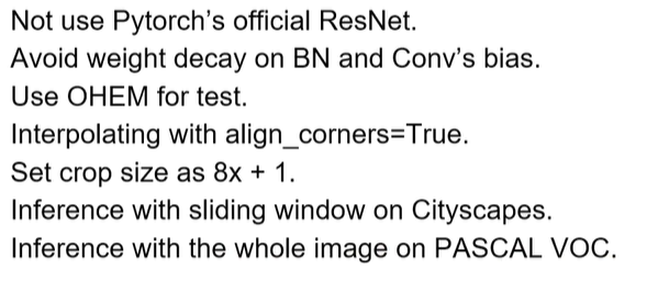
  Tricks for semantic segmentation：

  Bag of tricks for image classification with convolutional neural networks

  语义分割技巧:

因能力有限，讲了太多的论文，以前也没有过接触，感觉听不懂，仅作论文记录，待以后详看。

• 图像语义分割前沿进展

  面临挑战：

  ​ 大小各异、形状复杂、环境多变、类别众多——怎样用有限计算资源去理解无限复杂的真实世界

  计算机视觉发展：

  ​ SIFT、AlexNet、VggNet、ResNet、DenseNet——多尺度信息处理；

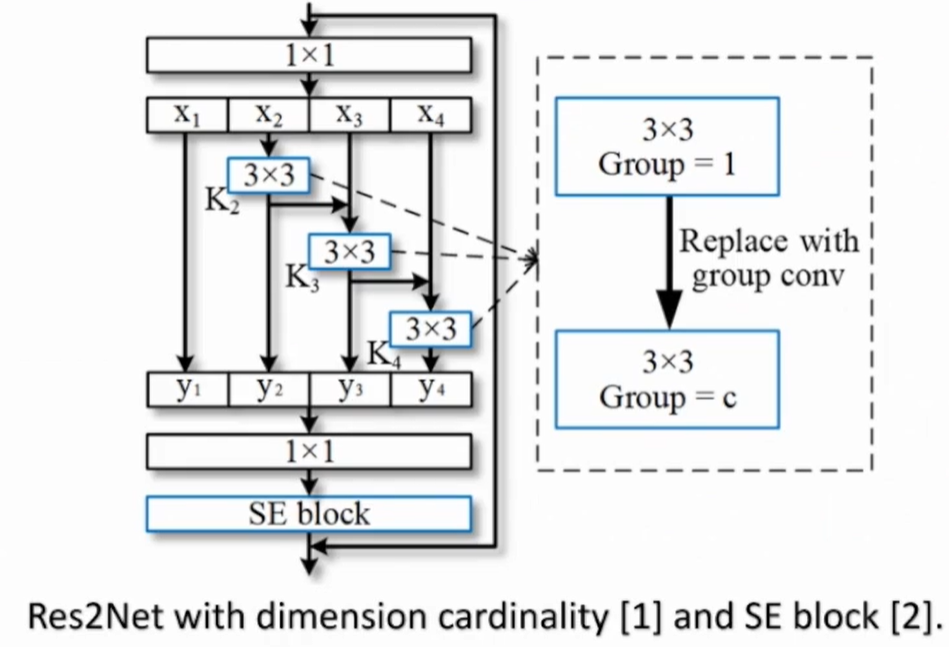
  卷积层提高特征提取性能：Res2Net：A New Multi-scale Backbone Architecture

  ​ 提供一种神经网络层类多尺度信息方面提取能力，可以更好提取不同尺度的信息，做出更好的决策，且计算量小，运行速度快。

池化层提高性能：细节+全局信息的提取

​ Non-local modules、Self-attention——计算消耗资源过大

​ Dilated convolution、Pyramid/global pooling——各向同性，不能获得各向异性信息

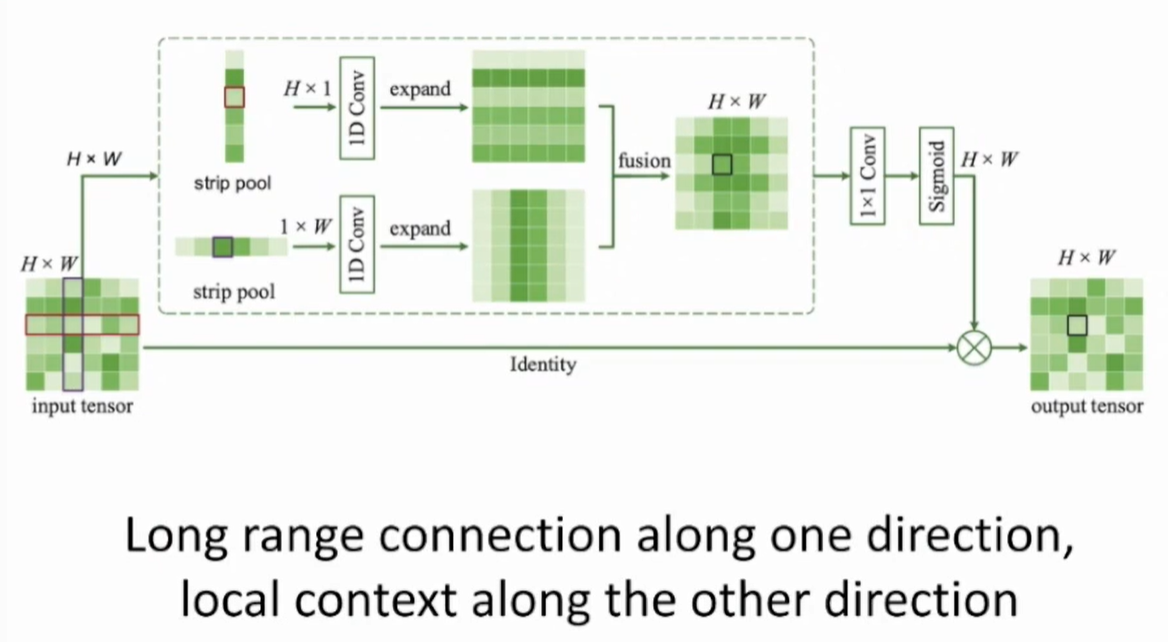
自适应池化、带状池化——Srtip Poolong（SP）模块：

​ 一个方向建立long range connection，另一个方向保持local context