NLP（二十九）一步一步，理解Self-Attention

  本文大部分内容翻译自Illustrated Self-Attention, Step-by-step guide to self-attention with illustrations and code，仅用于学习，如有翻译不当之处，敬请谅解！

什么是Self-Attention（自注意力机制）？

  如果你在想Self-Attention（自注意力机制）是否和Attention（注意力机制）相似，那么答案是肯定的。它们本质上属于同一个概念，拥有许多共同的数学运算。
  一个Self-Attention模块拥有n个输入，返回n个输出。这么模块里面发生了什么？从非专业角度看，Self-Attention（自注意力机制）允许输入之间互相作用（“self”部分），寻找出谁更应该值得注意（“attention”部分）。输出的结果是这些互相作用和注意力分数的聚合。

一步步理解Self-Attention

  理解分为以下几步：

1. 准备输入；
2. 初始化权重；
3. 获取key，query和value；
4. 为第1个输入计算注意力分数；
5. 计算softmax;
6. 将分数乘以values；
7. 对权重化后的values求和，得到输出1；
8. 对其余的输入，重复第4-7步。

注意：实际上，这些数学运算都是向量化的，也就是说，所有的输入都会一起经历这些数学运算。我们将会在后面的代码部分看到。

第一步：准备输入

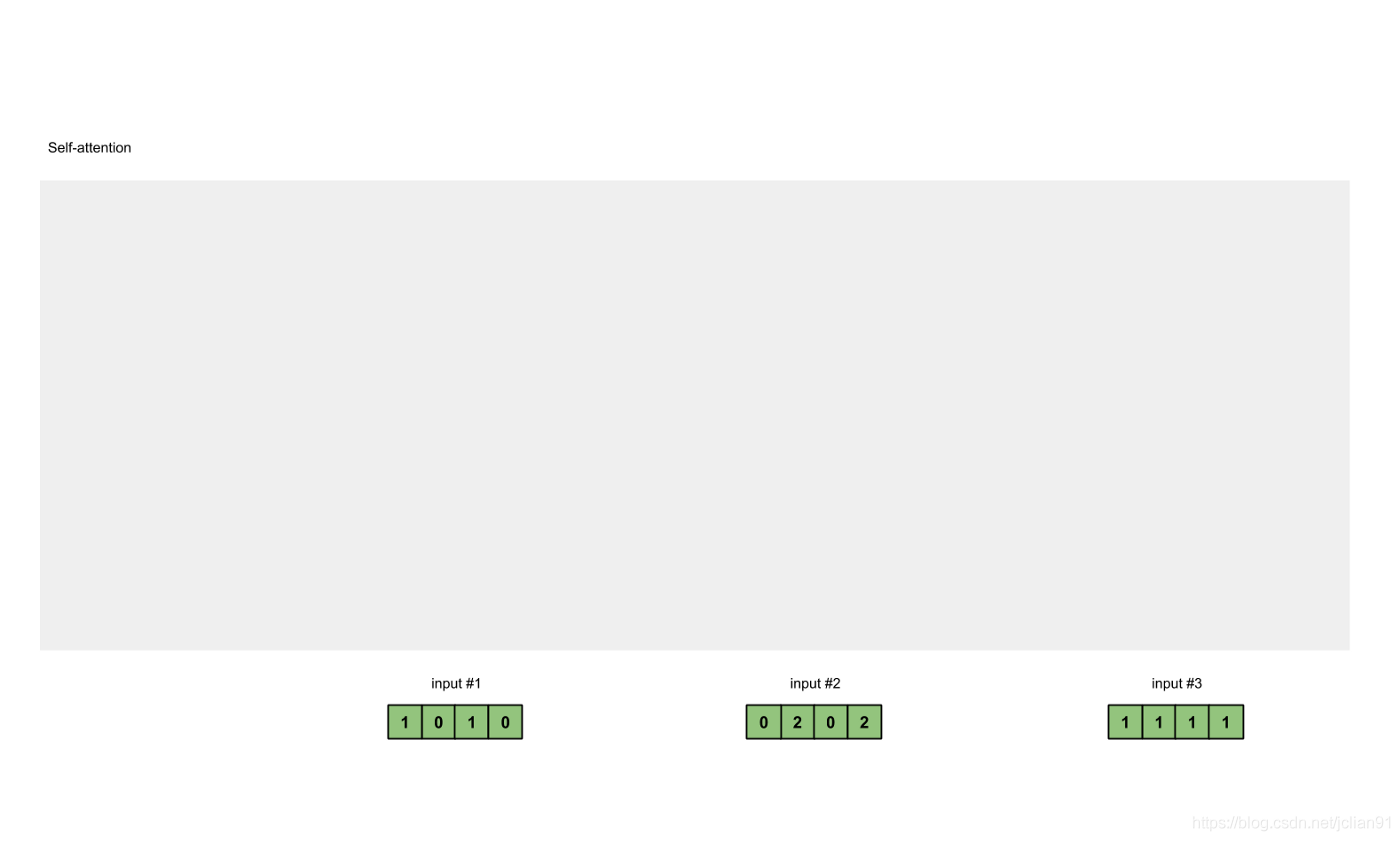
在这个教程中，我们从3个输入开始，每个输入的维数为4。

Input 1: [1, 0, 1, 0] 
Input 2: [0, 2, 0, 2]
Input 3: [1, 1, 1, 1]

第二步：初始化权重

  每个输入必须由三个表示（看下图）。这些输入被称作key（橙色），query（红色）value（紫色）。在这个例子中，我们假设我们想要的表示维数为3。因为每个输入的维数为4，这就意味着每个权重的形状为4×3。

注意：我们稍后会看到value的维数也是output的维数。

  为了获取这些表示，每个输入（绿色）会乘以一个权重的集合得到keys，乘以一个权重的集合得到queries，乘以一个权重的集合得到values。在我们的例子中，我们初始化三个权重的集合如下。
  key的权重：

[[0, 0, 1],
 [1, 1, 0],
 [0, 1, 0],
 [1, 1, 0]]

  query的权重：

[[1, 0, 1],
 [1, 0, 0],
 [0, 0, 1],
 [0, 1, 1]]

  value的权重：

[[0, 2, 0],
 [0, 3, 0],
 [1, 0, 3],
 [1, 1, 0]]

注意： 在神经网络设置中，这些权重通常都是一些小的数字，利用随机分布，比如Gaussian, Xavier and Kaiming分布，随机初始化。在训练开始前已经完成初始化。

第三步：获取key，query和value；

  现在我们有了3个权重的集合，让我们来给每个输入获取key，query和value。
  第1个输入的key表示：

               [0, 0, 1]
[1, 0, 1, 0] x [1, 1, 0] = [0, 1, 1]
               [0, 1, 0]
               [1, 1, 0]

  利用相同的权重集合获取第2个输入的key表示：

               [0, 0, 1]
[0, 2, 0, 2] x [1, 1, 0] = [4, 4, 0]
               [0, 1, 0]
               [1, 1, 0]

  利用相同的权重集合获取第3个输入的key表示：

               [0, 0, 1]
[1, 1, 1, 1] x [1, 1, 0] = [2, 3, 1]
               [0, 1, 0]
               [1, 1, 0]

  更快的方式是将这些运算用向量来描述：

               [0, 0, 1]
[1, 0, 1, 0]   [1, 1, 0]   [0, 1, 1]
[0, 2, 0, 2] x [0, 1, 0] = [4, 4, 0]
[1, 1, 1, 1]   [1, 1, 0]   [2, 3, 1]

  让我们用相同的操作来获取每个输入的value表示：

最后是query的表示：

               [1, 0, 1]
[1, 0, 1, 0]   [1, 0, 0]   [1, 0, 2]
[0, 2, 0, 2] x [0, 0, 1] = [2, 2, 2]
[1, 1, 1, 1]   [0, 1, 1]   [2, 1, 3]

注意：实际上，一个偏重向量也许会加到矩阵相乘后的结果。

第四步：为第1个输入计算注意力分数

  为了获取注意力分数，我们从输入1的query（红色）和所有keys（橙色）的点积开始。因为有3个key表示（这是由于我们有3个输入），我们得到3个注意力分数（蓝色）。

            [0, 4, 2]
[1, 0, 2] x [1, 4, 3] = [2, 4, 4]
            [1, 0, 1]

注意到我们只用了输入的query。后面我们会为其他的queries重复这些步骤。

第五步：计算softmax

  对这些注意力分数进行softmax函数运算（蓝色部分）。

softmax([2, 4, 4]) = [0.0, 0.5, 0.5]

第六步： 将分数乘以values

  将每个输入（绿色）的softmax作用后的注意力分数乘以各自对应的value（紫色）。这会产生3个向量（黄色）。在这个教程中，我们把它们称作权重化value。

1: 0.0 * [1, 2, 3] = [0.0, 0.0, 0.0]
2: 0.5 * [2, 8, 0] = [1.0, 4.0, 0.0]
3: 0.5 * [2, 6, 3] = [1.0, 3.0, 1.5]

第七步：对权重化后的values求和，得到输出1

  将权重后value按元素相加得到输出1：

  [0.0, 0.0, 0.0]
+ [1.0, 4.0, 0.0]
+ [1.0, 3.0, 1.5]
-----------------
= [2.0, 7.0, 1.5]

  产生的向量[2.0, 7.0, 1.5]（暗绿色）就是输出1，这是基于输入1的query表示与其它的keys，包括它自身的key互相作用的结果。

第八步：对输入2、3，重复第4-7步

  既然我们已经完成了输入1，我们重复步骤4-7能得到输出2和3。这个可以留给读者自己尝试，相信聪明的你可以做出来。

代码

  这里有PyTorch的实现代码，PyTorch是一个主流的Python深度学习框架。为了能够很好地使用代码片段中的@运算符, .T and None操作，请确保Python≥3.6，PyTorch ≥1.3.1。

1. 准备输入

import torch

x = [
  [1, 0, 1, 0], # Input 1
  [0, 2, 0, 2], # Input 2
  [1, 1, 1, 1]  # Input 3
 ]
x = torch.tensor(x, dtype=torch.float32)

2. 初始化权重

w_key = [
  [0, 0, 1],
  [1, 1, 0],
  [0, 1, 0],
  [1, 1, 0]
]
w_query = [
  [1, 0, 1],
  [1, 0, 0],
  [0, 0, 1],
  [0, 1, 1]
]
w_value = [
  [0, 2, 0],
  [0, 3, 0],
  [1, 0, 3],
  [1, 1, 0]
]
w_key = torch.tensor(w_key, dtype=torch.float32)
w_query = torch.tensor(w_query, dtype=torch.float32)
w_value = torch.tensor(w_value, dtype=torch.float32)

3. 获取key，query和value

keys = x @ w_key
querys = x @ w_query
values = x @ w_value

print(keys)
# tensor([[0., 1., 1.],
#         [4., 4., 0.],
#         [2., 3., 1.]])

print(querys)
# tensor([[1., 0., 2.],
#         [2., 2., 2.],
#         [2., 1., 3.]])

print(values)
# tensor([[1., 2., 3.],
#         [2., 8., 0.],
#         [2., 6., 3.]])

4. 为第1个输入计算注意力分数

attn_scores = querys @ keys.T

# tensor([[ 2.,  4.,  4.],  # attention scores from Query 1
#         [ 4., 16., 12.],  # attention scores from Query 2
#         [ 4., 12., 10.]]) # attention scores from Query 3

5. 计算softmax

from torch.nn.functional import softmax

attn_scores_softmax = softmax(attn_scores, dim=-1)
# tensor([[6.3379e-02, 4.6831e-01, 4.6831e-01],
#         [6.0337e-06, 9.8201e-01, 1.7986e-02],
#         [2.9539e-04, 8.8054e-01, 1.1917e-01]])

# For readability, approximate the above as follows
attn_scores_softmax = [
  [0.0, 0.5, 0.5],
  [0.0, 1.0, 0.0],
  [0.0, 0.9, 0.1]
]
attn_scores_softmax = torch.tensor(attn_scores_softmax)

6. 将分数乘以values

weighted_values = values[:,None] * attn_scores_softmax.T[:,:,None]

# tensor([[[0.0000, 0.0000, 0.0000],
#          [0.0000, 0.0000, 0.0000],
#          [0.0000, 0.0000, 0.0000]],
# 
#         [[1.0000, 4.0000, 0.0000],
#          [2.0000, 8.0000, 0.0000],
#          [1.8000, 7.2000, 0.0000]],
# 
#         [[1.0000, 3.0000, 1.5000],
#          [0.0000, 0.0000, 0.0000],
#          [0.2000, 0.6000, 0.3000]]])

7. 对权重化后的values求和，得到输出

outputs = weighted_values.sum(dim=0)

# tensor([[2.0000, 7.0000, 1.5000],  # Output 1
#         [2.0000, 8.0000, 0.0000],  # Output 2
#         [2.0000, 7.8000, 0.3000]]) # Output 3

注意：PyTorch已经提供了这个API，名字为nn.MultiheadAttention。但是，这个API需要你提供PyTorch的Tensor形式的key，value，query。还有，这个模块的输出会经历一个线性变换。

自己实现？

  以下是笔者自己写的部分。
  对于不熟悉PyTorch的读者来说，上述的向量操作理解起来有点困难，因此，笔者自己用简单的Python代码实现了一遍上述Self-Attention的过程。
  完整的Python代码如下：

# -*- coding: utf-8 -*-

from typing import List
import math
from pprint import pprint

x = [[1, 0, 1, 0], # Input 1
     [0, 2, 0, 2], # Input 2
     [1, 1, 1, 1]  # Input 3
    ]

w_key = [[0, 0, 1],
        [1, 1, 0],
        [0, 1, 0],
        [1, 1, 0]
        ]

w_query = [[1, 0, 1],
            [1, 0, 0],
            [0, 0, 1],
            [0, 1, 1]
          ]

w_value = [[0, 2, 0],
            [0, 3, 0],
            [1, 0, 3],
            [1, 1, 0]
          ]


# vector dot of two vectors
def vector_dot(list1: List[float or int], list2: List[float or int]) -> float or int:
    dot_sum = 0
    for element_i, element_j in zip(list1, list2):
        dot_sum += element_i * element_j

    return dot_sum


# get weights matrix by x, using matrix multiplication
def get_weights_matrix_by_x(x, weight_matrix):
    x_matrix = []
    for i in range(len(x)):
        x_row = []
        for j in range(len(weight_matrix[0])):
            x_row.append(vector_dot(x[i], [_[j] for _ in weight_matrix]))

        x_matrix.append(x_row)

    return x_matrix


# softmax function
def softmax(x: List[float or int]) -> List[float or int]:
    x_sum = sum([math.exp(_) for _ in x])
    return [math.exp(_)/x_sum for _ in x]


x_key = get_weights_matrix_by_x(x, w_key)
x_value = get_weights_matrix_by_x(x, w_value)
x_query = get_weights_matrix_by_x(x, w_query)
# print(x_key)
# print(x_value)
# print(x_query)

outputs = []
for query in x_query:
    score_list = [vector_dot(query, key) for key in x_key]
    softmax_score_list = softmax(score_list)

    weights_list = []
    for i in range(len(softmax_score_list)):
        weights = [softmax_score_list[i] * _ for _ in x_value[i]]
        weights_list.append(weights)

    output = []
    for j in range(len(weights_list[0])):
        output.append(sum([_[j] for _ in weights_list]))

    outputs.append(output)

pprint(outputs)

输出结果如下：

[[1.9366210616669624, 6.683105308334811, 1.5950684074995565],
 [1.9999939663351456, 7.9639915951322156, 0.0539764053125496],
 [1.9997046127769653, 7.759892254657784, 0.3583892946751152]]

总结

  本文主要讲述了如何一步一步来实现Self-Attention机制，对于想要自己实现算法的读者来说，值得一读。
  本文分享到此结束，感谢大家的阅读~