数模 06模拟退火
模拟退火
模拟退火算法(Simulate Anneal,SA)是一种通用概率演算法,用来在一个大的搜寻空间内找寻命题的最优解。模拟退火是由S.Kirkpatrick, C.D.Gelatt和M.P.Vecchi在1983年所发明的。V.Černý在1985年也独立发明此演算法。模拟退火算法是解决TSP问题的有效方法之一。
关于算法过程呢,这里不说了,和机器学习中的梯度下降算法差不多,挺简单的。今天晚上徒弟搞得我难受的,就说说matlab和python实现吧。
先说说matlab实现吧,是从一家培训机构学到的。


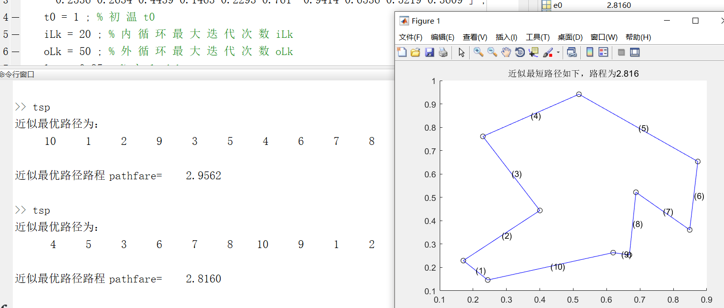
swap.m
function [ newpath , position ] = swap( oldpath , number )
% 对 oldpath 进 行 互 换 操 作
% number 为 产 生 的 新 路 径 的 个 数
% position 为 对 应 newpath 互 换 的 位 置
m = length( oldpath ) ; % 城 市 的 个 数
newpath = zeros( number , m ) ;
position = sort( randi( m , number , 2 ) , 2 ); % 随 机 产 生 交 换 的 位 置
for i = 1 : number
newpath( i , : ) = oldpath ;
% 交 换 路 径 中 选 中 的 城 市
newpath( i , position( i , 1 ) ) = oldpath( position( i , 2 ) ) ;
newpath( i , position( i , 2 ) ) = oldpath( position( i , 1 ) ) ;
end


pathfare.m
function [ objval ] = pathfare( fare , path )
% 计 算 路 径 path 的 代 价 objval
% path 为 1 到 n 的 排 列 ,代 表 城 市 的 访 问 顺 序 ;
% fare 为 代 价 矩 阵 , 且 为 方 阵 。
[ m , n ] = size( path ) ;
objval = zeros( 1 , m ) ;
for i = 1 : m
for j = 2 : n
objval( i ) = objval( i ) + fare( path( i , j - 1 ) , path( i , j ) ) ;
end
objval( i ) = objval( i ) + fare( path( i , n ) , path( i , 1 ) ) ;
end


distance.m
function [ fare ] = distance( coord )
% 根 据 各 城 市 的 距 离 坐 标 求 相 互 之 间 的 距 离
% fare 为 各 城 市 的 距 离 , coord 为 各 城 市 的 坐 标
[ v , m ] = size( coord ) ; % m 为 城 市 的 个 数
fare = zeros( m ) ;
for i = 1 : m % 外 层 为 行
for j = i : m % 内 层 为 列
fare( i , j ) = ( sum( ( coord( : , i ) - coord( : , j ) ) .^ 2 ) ) ^ 0.5 ;
fare( j , i ) = fare( i , j ) ; % 距 离 矩 阵 对 称
end
end


myplot.m
function [ ] = myplot( path , coord , pathfar )
% 做 出 路 径 的 图 形
% path 为 要 做 图 的 路 径 ,coord 为 各 个 城 市 的 坐 标
% pathfar 为 路 径 path 对 应 的 费 用
len = length( path ) ;
clf ;
hold on ;
title( [ '近似最短路径如下,路程为' , num2str( pathfar ) ] ) ;
plot( coord( 1 , : ) , coord( 2 , : ) , 'ok');
pause( 0.4 ) ;
for ii = 2 : len
plot( coord( 1 , path( [ ii - 1 , ii ] ) ) , coord( 2 , path( [ ii - 1 , ii ] ) ) , '-b');
x = sum( coord( 1 , path( [ ii - 1 , ii ] ) ) ) / 2 ;
y = sum( coord( 2 , path( [ ii - 1 , ii ] ) ) ) / 2 ;
text( x , y , [ '(' , num2str( ii - 1 ) , ')' ] ) ;
pause( 0.4 ) ;
end
plot( coord( 1 , path( [ 1 , len ] ) ) , coord( 2 , path( [ 1 , len ] ) ) , '-b' ) ;
x = sum( coord( 1 , path( [ 1 , len ] ) ) ) / 2 ;
y = sum( coord( 2 , path( [ 1 , len ] ) ) ) / 2 ;
text( x , y , [ '(' , num2str( len ) , ')' ] ) ;
pause( 0.4 ) ;
hold off ;


clear;
% 程 序 参 数 设 定
Coord = ... % 城 市 的 坐 标 Coordinates
[ 0.6683 0.6195 0.4    0.2439 0.1707 0.2293 0.5171 0.8732 0.6878 0.8488 ; ...
  0.2536 0.2634 0.4439 0.1463 0.2293 0.761  0.9414 0.6536 0.5219 0.3609 ] ;
t0 = 1 ; % 初 温 t0
iLk = 20 ; % 内 循 环 最 大 迭 代 次 数 iLk
oLk = 50 ; % 外 循 环 最 大 迭 代 次 数 oLk
lam = 0.95 ; % λ lambda
istd = 0.001 ; % 若 内 循 环 函 数 值 方 差 小 于 istd 则 停 止
ostd = 0.001 ; % 若 外 循 环 函 数 值 方 差 小 于 ostd 则 停 止
ilen = 5 ; % 内 循 环 保 存 的 目 标 函 数 值 个 数
olen = 5 ; % 外 循 环 保 存 的 目 标 函 数 值 个 数
% 程 序 主 体
m = length( Coord ) ; % 城 市 的 个 数 m
fare = distance( Coord ) ; % 路 径 费 用 fare
path = 1 : m ; % 初 始 路 径 path
pathfar = pathfare( fare , path ) ; % 路 径 费 用 path fare
ores = zeros( 1 , olen ) ; % 外 循 环 保 存 的 目 标 函 数 值
e0 = pathfar ; % 能 量 初 值 e0
t = t0 ; % 温 度 t
for out = 1 : oLk % 外 循 环 模 拟 退 火 过 程
ires = zeros( 1 , ilen ) ; % 内 循 环 保 存 的 目 标 函 数 值
for in = 1 : iLk % 内 循 环 模 拟 热 平 衡 过 程
[ newpath , v ] = swap( path , 1 ) ; % 产 生 新 状 态
e1 = pathfare( fare , newpath ) ; % 新 状 态 能 量
% Metropolis 抽 样 稳 定 准 则
r = min( 1 , exp( - ( e1 - e0 ) / t ) ) ;
if rand < r
path = newpath ; % 更 新 最 佳 状 态
e0 = e1 ;
end
ires = [ ires( 2 : end ) e0 ] ; % 保 存 新 状 态 能 量
% 内 循 环 终 止 准 则 :连 续 ilen 个 状 态 能 量 波 动 小 于 istd
if std( ires , 1 ) < istd
break ;
end
end
ores = [ ores( 2 : end ) e0 ] ; % 保 存 新 状 态 能 量
% 外 循 环 终 止 准 则 :连 续 olen 个 状 态 能 量 波 动 小 于 ostd
if std( ores , 1 ) < ostd
break ;
end
t = lam * t ;
end
pathfar = e0 ;
% 输 入 结 果
fprintf( '近似最优路径为:\n ' )
%disp( char( [ path , path(1) ] + 64 ) ) ;
disp(path)
fprintf( '近似最优路径路程\tpathfare=' ) ;
disp( pathfar ) ;
myplot( path , Coord , pathfar ) ;
操作:
最后一个文件中,改变
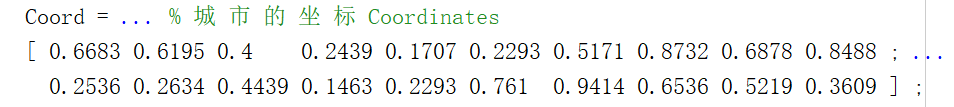
注意上下对应它们的坐标x,y轴,比如第一个是:(0.6683,0.2536)
将上述运行结束之后,结果为:
至于梯度下降算法可以看我的其他博客,里面有介绍。
下面说说python的模拟退火算法实现
import numpy as np
import matplotlib.pyplot as plt
import random


class SA(object):

    def __init__(self, interval, tab='min', T_max=10000, T_min=1, iterMax=1000, rate=0.95):
        self.interval = interval  # 给定状态空间 - 即待求解空间
        self.T_max = T_max  # 初始退火温度 - 温度上限
        self.T_min = T_min  # 截止退火温度 - 温度下限
        self.iterMax = iterMax  # 定温内部迭代次数
        self.rate = rate  # 退火降温速度
        #############################################################
        self.x_seed = random.uniform(interval[0], interval[1])  # 解空间内的种子
        self.tab = tab.strip()  # 求解最大值还是最小值的标签: 'min' - 最小值;'max' - 最大值
        #############################################################
        self.solve()  # 完成主体的求解过程
        self.display()  # 数据可视化展示

    def solve(self):
        temp = 'deal_' + self.tab  # 采用反射方法提取对应的函数
        if hasattr(self, temp):
            deal = getattr(self, temp)
        else:
            exit('>>>tab标签传参有误:"min"|"max"<<<')
        x1 = self.x_seed
        T = self.T_max
        while T >= self.T_min:
            for i in range(self.iterMax):
                f1 = self.func(x1)
                delta_x = random.random() * 2 - 1
                if x1 + delta_x >= self.interval[0] and x1 + delta_x <= self.interval[1]:  # 将随机解束缚在给定状态空间内
                    x2 = x1 + delta_x
                else:
                    x2 = x1 - delta_x
                f2 = self.func(x2)
                delta_f = f2 - f1
                x1 = deal(x1, x2, delta_f, T)
            T *= self.rate
        self.x_solu = x1  # 提取最终退火解

    def func(self, x):  # 状态产生函数 - 即待求解函数
        value = np.sin(x ** 2) * (x ** 2 - 5 * x)
        return value

    def p_min(self, delta, T):  # 计算最小值时,容忍解的状态迁移概率
        probability = np.exp(-delta / T)
        return probability

    def p_max(self, delta, T):
        probability = np.exp(delta / T)  # 计算最大值时,容忍解的状态迁移概率
        return probability

    def deal_min(self, x1, x2, delta, T):
        if delta < 0:  # 更优解
            return x2
        else:  # 容忍解
            P = self.p_min(delta, T)
            if P > random.random():
                return x2
            else:
                return x1

    def deal_max(self, x1, x2, delta, T):
        if delta > 0:  # 更优解
            return x2
        else:  # 容忍解
            P = self.p_max(delta, T)
            if P > random.random():
                return x2
            else:
                return x1

    def display(self):
        print('seed: {}\nsolution: {}'.format(self.x_seed, self.x_solu))
        plt.figure(figsize=(6, 4))
        x = np.linspace(self.interval[0], self.interval[1], 300)
        y = self.func(x)
        plt.plot(x, y, 'g-', label='function')
        plt.plot(self.x_seed, self.func(self.x_seed), 'bo', label='seed')
        plt.plot(self.x_solu, self.func(self.x_solu), 'r*', label='solution')
        plt.title('solution = {}'.format(self.x_solu))
        plt.xlabel('x')
        plt.ylabel('y')
        plt.legend()
        plt.savefig('SA.png', dpi=500)
        plt.show()
        plt.close()


if __name__ == '__main__':
    SA([-5, 5], 'min')    #这里可以调整
中间的函数是需要根据实际问题修改的参数
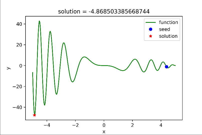
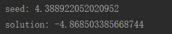
这是输出结果。seed表示随机种子
上面类似于梯度下降了,下面谈一谈旅行商问题。
需要三个文件
# -*- coding: utf-8 -*-

import random
from Life import Life

class GA(object):
      """遗传算法类"""
      def __init__(self, aCrossRate, aMutationRate, aLifeCount, aGeneLength, aMatchFun = lambda life : 1):
            self.crossRate = aCrossRate               #交叉概率
            self.mutationRate = aMutationRate         #突变概率
            self.lifeCount = aLifeCount               #种群数量,就是每次我们在多少个城市序列里筛选,这里初始化为100
            self.geneLength = aGeneLength             #其实就是城市数量
            self.matchFun = aMatchFun                 #适配函数
            self.lives = []                           #种群
            self.best = None                          #保存这一代中最好的个体
            self.generation = 1                       #一开始的是第一代
            self.crossCount = 0                       #一开始还没交叉过,所以交叉次数是0
            self.mutationCount = 0                    #一开始还没变异过,所以变异次数是0
            self.bounds = 0.0                         #适配值之和,用于选择时计算概率

            self.initPopulation()                     #初始化种群


      def initPopulation(self):
            """初始化种群"""
            self.lives = []
            for i in range(self.lifeCount):
                  #gene = [0,1,…… ,self.geneLength-1]
                  #事实就是0到33
                  gene = range(self.geneLength)
                  #将0到33序列的所有元素随机排序得到一个新的序列
                  random.shuffle(gene)
                  #Life这个类就是一个基因序列,初始化life的时候,两个参数,一个是序列gene,一个是这个序列的初始适应度值
                  # 因为适应度值越大,越可能被选择,所以一开始种群里的所有基因都被初始化为-1
                  life = Life(gene)
                  #把生成的这个基因序列life填进种群集合里
                  self.lives.append(life)


      def judge(self):
            """评估,计算每一个个体的适配值"""
            # 适配值之和,用于选择时计算概率
            self.bounds = 0.0
            #假设种群中的第一个基因被选中
            self.best = self.lives[0]
            for life in self.lives:
                  life.score = self.matchFun(life)
                  self.bounds += life.score
                  #如果新基因的适配值大于原先的best基因,就更新best基因
                  if self.best.score < life.score:
                        self.best = life


      def cross(self, parent1, parent2):
            """交叉"""
            index1 = random.randint(0, self.geneLength - 1)
            index2 = random.randint(index1, self.geneLength - 1)
            tempGene = parent2.gene[index1:index2]                      #交叉的基因片段
            newGene = []
            p1len = 0
            for g in parent1.gene:
                  if p1len == index1:
                        newGene.extend(tempGene)                               #插入基因片段
                        p1len += 1
                  if g not in tempGene:
                        newGene.append(g)
                        p1len += 1
            self.crossCount += 1
            return newGene


      def  mutation(self, gene):
            """突变"""
            #相当于取得0到self.geneLength - 1之间的一个数,包括0和self.geneLength - 1
            index1 = random.randint(0, self.geneLength - 1)
            index2 = random.randint(0, self.geneLength - 1)
            #把这两个位置的城市互换
            gene[index1], gene[index2] = gene[index2], gene[index1]
            #突变次数加1
            self.mutationCount += 1
            return gene


      def getOne(self):
            """选择一个个体"""
            #产生0到(适配值之和)之间的任何一个实数
            r = random.uniform(0, self.bounds)
            for life in self.lives:
                  r -= life.score
                  if r <= 0:
                        return life

            raise Exception("选择错误", self.bounds)


      def newChild(self):
            """产生新后的"""
            parent1 = self.getOne()
            rate = random.random()

            #按概率交叉
            if rate < self.crossRate:
                  #交叉
                  parent2 = self.getOne()
                  gene = self.cross(parent1, parent2)
            else:
                  gene = parent1.gene

            #按概率突变
            rate = random.random()
            if rate < self.mutationRate:
                  gene = self.mutation(gene)

            return Life(gene)


      def next(self):
            """产生下一代"""
            self.judge()#评估,计算每一个个体的适配值
            newLives = []
            newLives.append(self.best)#把最好的个体加入下一代
            while len(newLives) < self.lifeCount:
                  newLives.append(self.newChild())
            self.lives = newLives
            self.generation += 1
# -*- encoding: utf-8 -*-


SCORE_NONE = -1

class Life(object):
      """个体类"""
      def __init__(self, aGene = None):
            self.gene = aGene
            self.score = SCORE_NONE
# -*- encoding: utf-8 -*-

import random
import math
import Tkinter
from GA import GA

class TSP(object):
      def __init__(self, aLifeCount = 100,):
            self.initCitys()
            self.lifeCount = aLifeCount
            self.ga = GA(aCrossRate = 0.7,
                  aMutationRate = 0.02,
                  aLifeCount = self.lifeCount,
                  aGeneLength = len(self.citys),
                  aMatchFun = self.matchFun())


      def initCitys(self):
            self.citys = []
            #这个文件里是34个城市的经纬度
            f=open("distanceMatrix.txt","r")
            while True:
                  #一行一行读取
                  loci = str(f.readline())
                  if loci:
                        pass  # do something here
                  else:
                        break
                  #用readline读取末尾总会有一个回车,用replace函数删除这个回车
                  loci = loci.replace("\n", "")
                  #按照tab键分割
                  loci=loci.split("\t")
                  # 中国34城市经纬度读入citys
                  self.citys.append((float(loci[1]),float(loci[2]),loci[0]))

      #order是遍历所有城市的一组序列,如[1,2,3,7,6,5,4,8……]
      #distance就是计算这样走要走多长的路
      def distance(self, order):
            distance = 0.0
            #i从-1到32,-1是倒数第一个
            for i in range(-1, len(self.citys) - 1):
                  index1, index2 = order[i], order[i + 1]
                  city1, city2 = self.citys[index1], self.citys[index2]
                  distance += math.sqrt((city1[0] - city2[0]) ** 2 + (city1[1] - city2[1]) ** 2)

            return distance

      #适应度函数,因为我们要从种群中挑选距离最短的,作为最优解,所以(1/距离)最长的就是我们要求的
      def matchFun(self):
            return lambda life: 1.0 / self.distance(life.gene)


      def run(self, n = 0):
            while n > 0:
                  self.ga.next()
                  distance = self.distance(self.ga.best.gene)
                  print (("%d : %f") % (self.ga.generation, distance))
                  print self.ga.best.gene
                  n -= 1
            print "经过%d次迭代,最优解距离为:%f"%(self.ga.generation, distance)
            print "遍历城市顺序为:",
            # print "遍历城市顺序为:", self.ga.best.gene
            #打印出我们挑选出的这个序列中
            for i in self.ga.best.gene:
                  print self.citys[i][2],

def main():
      tsp = TSP()
      tsp.run(100)


if __name__ == '__main__':
      main()
还需要城市经纬度
北京    116.46    39.92
天津    117.2    39.13
上海    121.48    31.22
重庆    106.54    29.59
拉萨    91.11    29.97
乌鲁木齐    87.68    43.77
银川    106.27    38.47
呼和浩特    111.65    40.82
南宁    108.33    22.84
哈尔滨    126.63    45.75
长春    125.35    43.88
沈阳    123.38    41.8
石家庄    114.48    38.03
太原    112.53    37.87
西宁    101.74    36.56
济南    117    36.65
郑州    113.6    34.76
南京    118.78    32.04
合肥    117.27    31.86
杭州    120.19    30.26
福州    119.3    26.08
南昌    115.89    28.68
长沙    113    28.21
武汉    114.31    30.52
广州    113.23    23.16
台北    121.5    25.05
海口    110.35    20.02
兰州    103.73    36.03
西安    108.95    34.27
成都    104.06    30.67
贵阳    106.71    26.57
昆明    102.73    25.04
香港    114.1    22.2
澳门    113.33    22.13
over,注意得下载tkinter库,python代码是2的,转3 需要一些代码替换,累了,溜了。

 浙公网安备 33010602011771号