Stanford_CS224W----Graph Neural Networks

Stanford_CS224W----Graph Neural Networks

这节课讲解了GNN中的一些普遍概念，为后面讲特定的GCN GraphSage等奠定基础

Deep learning for Graphs

在对图做深度学习时，主要的思想是，使用节点序无关的函数对图进行处理（当然有也有特例）。在这个思想上，其他的CNN，RNN甚至MLPs不能作用到图上。

解决思想：Node's neighborhood defines a computation graph---节点的领域构成了一个计算图，基于本地网络邻域生成节点嵌入

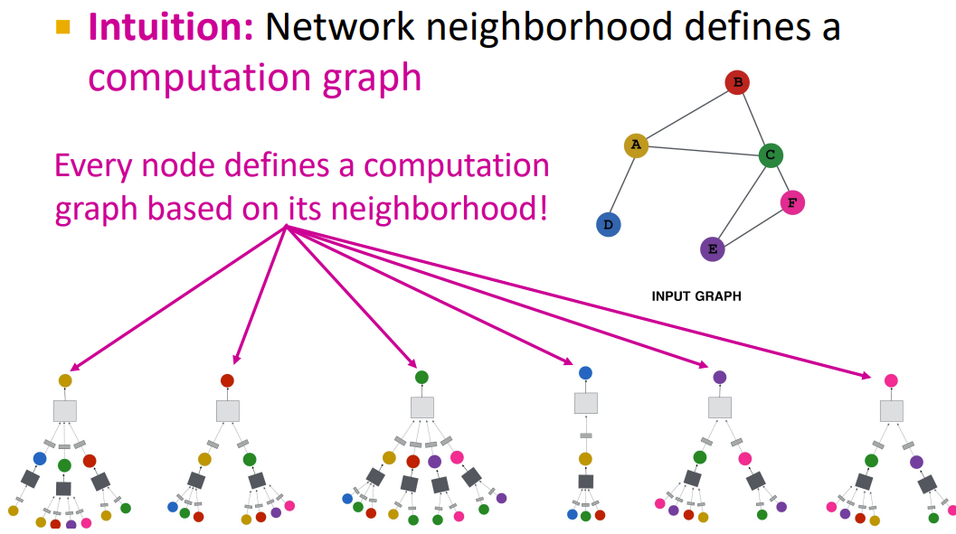
可以看到上午的矩形是灰色的，那里体现出了每种GNN方法的差异。

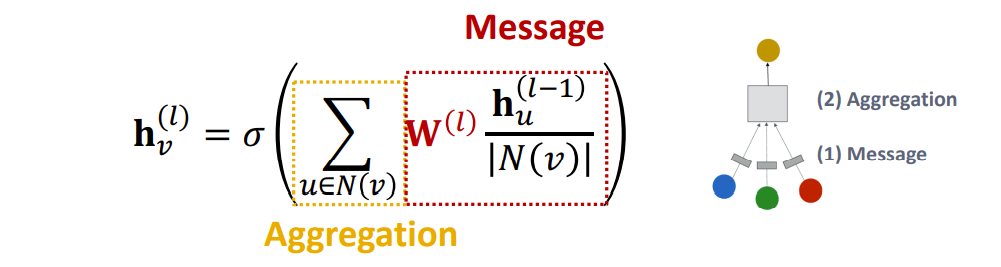
A Single GNN Layer

分为message计算和message聚合

• Message: each node computes a message

\[\mathbf{m}_{u}^{(l)}=\operatorname{MSG}^{(l)}\left(\mathbf{h}_{u}^{(l-1)}\right), u \in\{N(v) \cup v\} \]

• Aggregation: aggregate messages from neighbors

\[\mathbf{h}_{v}^{(l)}=\mathrm{AGG}^{(l)}\left(\left\{\mathbf{m}_{u}^{(l)}, u \in N(v)\right\}, \mathbf{m}_{v}^{(l)}\right) \]

GCN

• Message

\[\mathbf{m}_{u}^{(l)}=\frac{1}{|N(v)|} \mathbf{W}^{(l)} \mathbf{h}_{u}^{(l-1)} \]

• Aggregation

\[\mathbf{h}_{v}^{(l)}=\sigma\left(\operatorname{Sum}\left(\left\{\mathbf{m}_{u}^{(l)}, u \in N(v)\right\}\right)\right) \]

GraphSAGE

\[\mathbf{h}_{v}^{(l)}=\sigma\left(\mathbf{W}^{(l)} \cdot \operatorname{CONCAT}\left(\mathbf{h}_{v}^{(l-1)}, \operatorname{AGG}\left(\left\{\mathbf{h}_{u}^{(l-1)}, \forall u \in N(v)\right\}\right)\right)\right) \]

其中AGG代表了许多种计算message的方法，以下都是可用的

• Mean

\[AGG=\sum_{u \in N(v)} \frac{\mathbf{h}_{u}^{(l-1)}}{|N(v)|} \]

• Pool: Transform neighbor vectors and apply symmetric vector function Mean(⋅) or Max(⋅)

\[\mathrm{AGG}=\operatorname{Mean}\left(\left\{\operatorname{MLP}\left(\mathbf{h}_{u}^{(l-1)}\right), \forall u \in N(v)\right\}\right) \]

• LSTM

\[\mathrm{AGG}=\operatorname{LSTM}\left(\left[\mathbf{h}_{u}^{(l-1)}, \forall u \in \pi(N(v))\right]\right) \]

• ℓ2 Normalization 可选的正则化

GAT

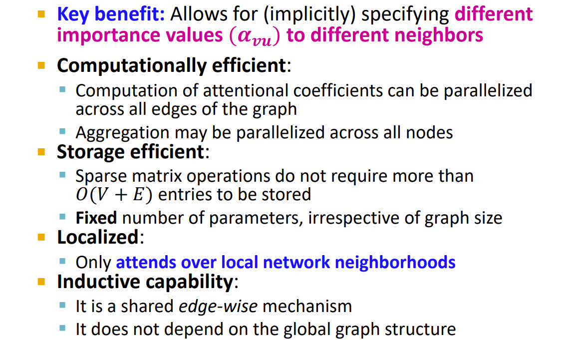
\[\mathbf{h}_{v}^{(l)}=\sigma\left(\sum_{u \in N(v)} \alpha_{v u} \mathbf{W}^{(l)} \mathbf{h}_{u}^{(l-1)}\right) \]

其中的\(\alpha_{v u}\)代表了u->v的消息的权重大小，注意这些权重是训练过程中的副产物

• Multi-head attention 稳定了注意力机制的学习过程,初始化不同的注意力权重，它们落到不同的优化区域中

\[\mathbf{h}_{v}^{(l)}[1]=\sigma\left(\sum_{u \in N(v)} \alpha_{v u}^{1} \mathbf{W}^{(l)} \mathbf{h}_{u}^{(l-1)}\right) \\ \mathbf{h}_{v}^{(l)}[1]=\sigma\left(\sum_{u \in N(v)} \alpha_{v u}^{2} \mathbf{W}^{(2)} \mathbf{h}_{u}^{(l-1)}\right) \\ \mathbf{h}_{v}^{(l)}[1]=\sigma\left(\sum_{u \in N(v)} \alpha_{v u}^{3} \mathbf{W}^{(3)} \mathbf{h}_{u}^{(l-1)}\right) \\ \]

benefit：

practice in GNN

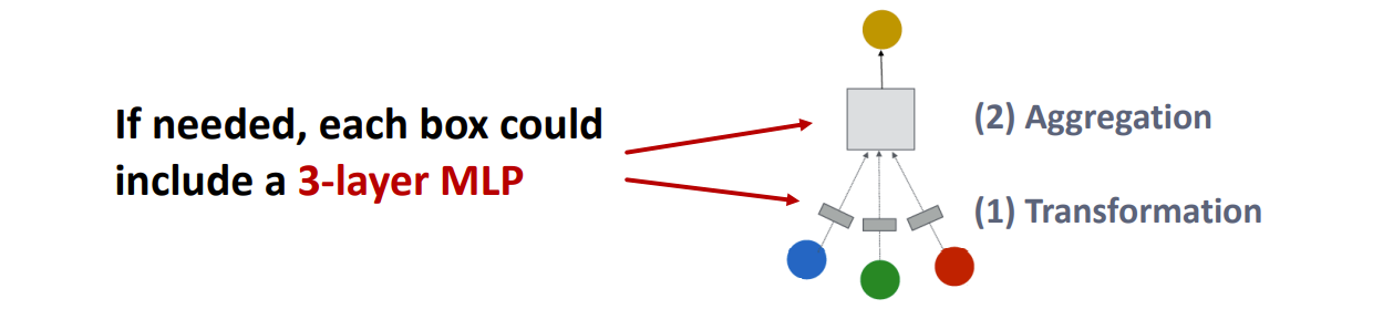
How to make a shallow GNN more expressive?

Solution 1: Increase the expressive power within each GNN layer

在每一层的内部添加一些多层感知机进行计算

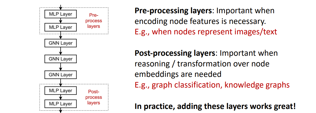
Solution 2: Add layers that do not pass messages

添加一些多层感知机的层

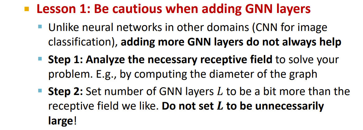
What if my problem still requires many GNN layers

The Over-smoothing Problem

Stack many GNN layers -》 nodes will have highly-overlapped receptive fields -》 node embeddings will be highly similar -》 suffer from the over-smoothing problem

危害：所有的节点嵌入都收敛到相同的值。

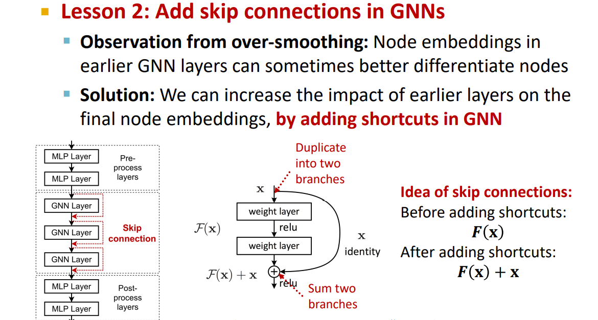
Solution 1

Solution 2

Augment Graphs

有些时候输入的图需要进行处理，并不是可计算的图。会碰到以下这些情况：

• Features
  • 输入的图缺少特征 -> 自定义特征
• Graph tructure
  • 图稀疏->消息传递十分低效->添加虚拟节点或者边
  • 图稠密->消息传递花费多->进行邻居采样
  • 图巨大->难以使用GPU计算->对子图进行采样

解决方法

feature augmentation

• 图没有特征

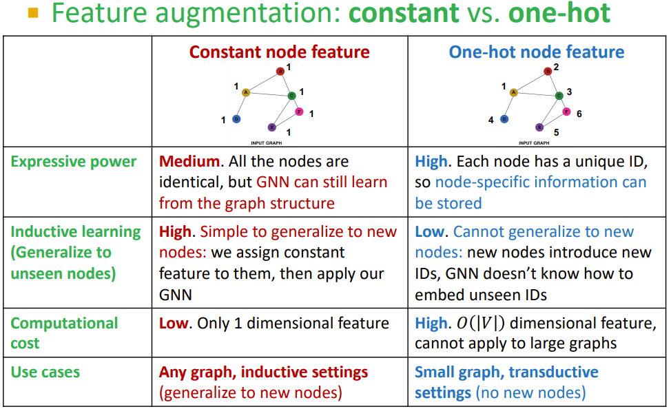
  • 两种方法及对比
    

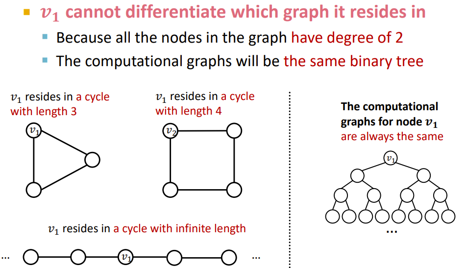
• 部分特定的结构难以被GNN学习：比如在环中的点，因为计算树结构相同（如果没有点的特定特征），无法得出3环形图和4环形图的区别。
  

  一些可以用的方法

  • Node degree
  • Clustering coefficient
  • PageRank
  • Centrality
  • 其他传统机器学习的特点

Add Virual Nodes or edges

• 添加虚拟边

  • 通常的方法是连接2-hop的点(在二分图类具有解释作用)
  • 在邻接矩阵中为\(A+A^2\)

• 添加虚拟点

  • 添加一些能连接所有点的虚拟点，因为在某些情况下，相聚很远的两个点也会产生联系。

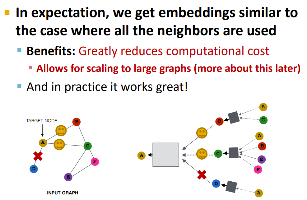
Neighborhood Samping

希望采样的邻居，在后续的聚合时，能使用所有的节点

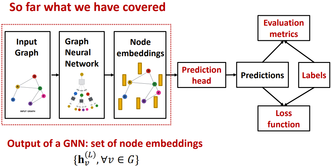
GNN Training Pipeline

目前学习了节点的嵌入，接下来会对点，边，整图的应用进行分类讲解。

Prediction heads

• Node-level tasks
• Edge-level tasks
• Graph-level tasks

Node-level tasks

可以直接使用节点嵌入进行计算

\[\widehat{\boldsymbol{y}}_{v}=\operatorname{Head}_{\text {node }}\left(\mathbf{h}_{v}^{(L)}\right)=\mathbf{W}^{(H)} \mathbf{h}_{v}^{(L)} \]

其中\(W\)为学习的参数，讲节点嵌入参数变成需要的预测值，当然这只是一个简单的例子。

Edge-level tasks

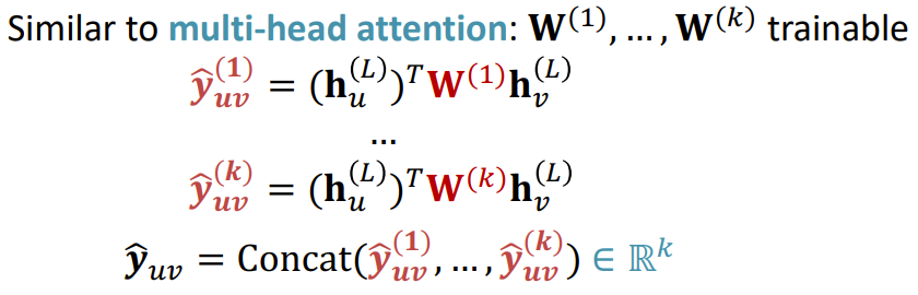
假设做一个k-way多分类。

\[\widehat{y}_{\boldsymbol{u v}}=\operatorname{Head}_{\mathrm{edg} e}\left(\mathbf{h}_{u}^{(L)}, \mathbf{h}_{v}^{(L)}\right) \]

• Concatenation + Linear
  • \(\widehat{y}_{uv}=\operatorname{Linear}\left(\operatorname{Concat}\left(\mathbf{h}_{u}^{(L)},\mathbf{h}_{v}^{(L)}\right)\right)\)
• Dot product
  • \(\widehat{y}_{\boldsymbol{u} v}=\left(\mathbf{h}_{u}^{(L)}\right)^{T} \mathbf{h}_{v}^{(L)}\)
  • Applying to k-way prediction
    

Graph-level tasks

对所有的节点的嵌入向量进行处理，不同的方法对应不同的函数。

\[\widehat{y}_{G}=\operatorname{Head}_{\operatorname{graph}}\left(\left\{\mathbf{h}_{v}^{(L)} \in \mathbb{R}^{d}, \forall v \in G\right\}\right) \]

• Global mean pooling
  • \(\widehat{y}_{G}=\operatorname{Mean}\left(\left\{\mathbf{h}_{v}^{(L)} \in \mathbb{R}^{d}, \forall v \in G\right\}\right)\)
• Global max pooling
  • \(\widehat{y}_{G}=\operatorname{Max}\left(\left\{\mathbf{h}_{v}^{(L)} \in \mathbb{R}^{d}, \forall v \in G\right\}\right)\)
• Global sum pooling
  • \(\widehat{y}_{G}=\operatorname{Sum}\left(\left\{\mathbf{h}_{v}^{(L)} \in \mathbb{R}^{d}, \forall v \in G\right\}\right)\)

根据不同的应用和图需要的特点，选择不同的方法

Issue：在pooling中会存在信息的丢失

A solution: hierarchical--DiffPool

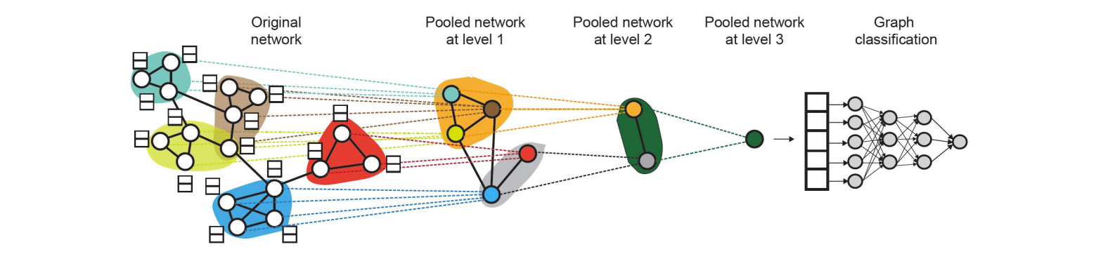
每层都有两个神经网络

• GNN A: Compute node embeddings
• GNN B: Compute the cluster that a node belongs to

process

• Use clustering assignments from GNN B to aggregate node embeddings generated by GNN A
• Create a single new node for each cluster, maintaining edges between clusters to generated a new pooled network

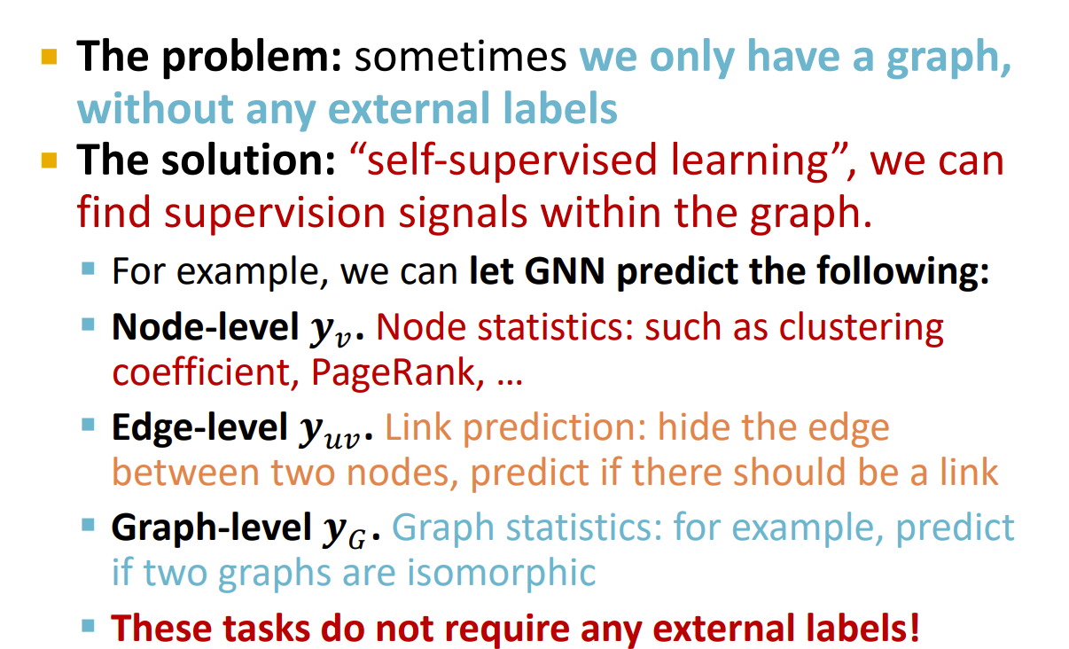
Prediction & Label

Supervised Labels On Graphs

Training Loss

对于不同的任务有不同的损失
Classification Loss

\[\mathrm{CE}\left({y}^{(i)}, \widehat{{y}}^{(i)}\right)=-\sum_{j=1}^{K} {y}_{j}^{(i)} \log \left(\widehat{{y}}_{j}^{(i)}\right) \]

\[\operatorname{Loss}=\sum_{i=1}^{N} \operatorname{CE}\left({y}^{(i)}, \widehat{{y}}^{(i)}\right) \]

Regression Loss

\[\operatorname{MSE}\left({y}^{(i)}, \widehat{{y}}^{(i)}\right)=\sum_{j=1}^{K}\left({y}_{j}^{(i)}-\widehat{{y}}_{j}^{(i)}\right)^{2} \]

\[\operatorname{LosS}=\sum_{i=1}^{N} \operatorname{MSE}\left({y}^{(i)}, \widehat{{y}}^{(i)}\right) \]

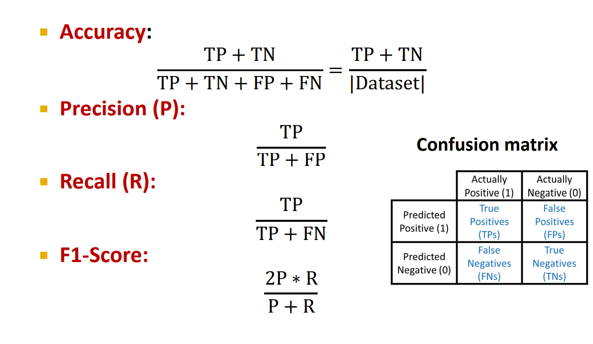
Evaluation Metrics

和常规的评估矩阵一样

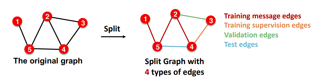
Dataset Split

对于图级别的训练集和验证集的分裂和其他神经网络一样，不再赘述。

Transductive and Inductive

直推式和归纳式，

node

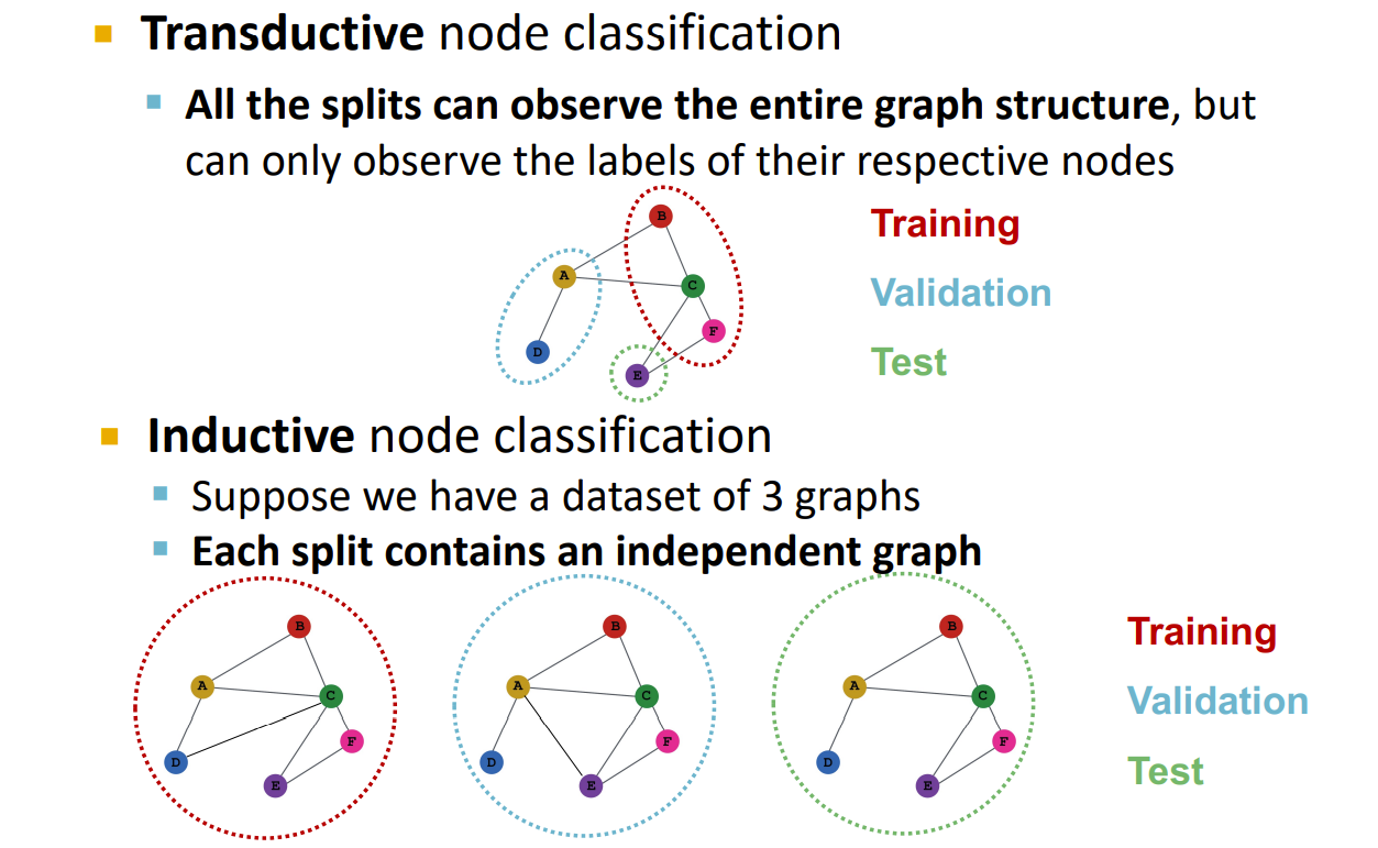
Link

Pytorch yyds。