

技术干货 | 基于MindSpore更好的理解Focal Loss
摘要:Focal Loss,是 Kaiming 大神团队在他们的论文Focal Loss for Dense Object Detection提出来的损失函数,利用它改善了图像物体检测的效果。
今天更新一下恺明大神的Focal Loss,它是 Kaiming 大神团队在他们的论文Focal Loss for Dense Object Detection提出来的损失函数,利用它改善了图像物体检测的效果。ICCV2017RBG和Kaiming大神的新作(https://arxiv.org/pdf/1708.02002.pdf)。
- 使用场景
最近一直在做人脸表情相关的方向,这个领域的 DataSet 数量不大,而且往往存在正负样本不均衡的问题。一般来说,解决正负样本数量不均衡问题有两个途径:
1. 设计采样策略,一般都是对数量少的样本进行重采样
2. 设计 Loss,一般都是对不同类别样本进行权重赋值
我两种策略都使用过,本文讲的是第二种策略中的 Focal Loss。

论文分析
我们知道object detection按其流程来说,一般分为两大类。一类是two stage detector(如非常经典的Faster R-CNN,RFCN这样需要region proposal的检测算法),第二类则是one stage detector(如SSD、YOLO系列这样不需要region proposal,直接回归的检测算法)。
对于第一类算法可以达到很高的准确率,但是速度较慢。虽然可以通过减少proposal的数量或降低输入图像的分辨率等方式达到提速,但是速度并没有质的提升。
对于第二类算法速度很快,但是准确率不如第一类。
所以目标就是:focal loss的出发点是希望one-stage detector可以达到two-stage detector的准确率,同时不影响原有的速度。
So,Why?and result?
这是什么原因造成的呢?the Reason is:Class Imbalance(正负样本不平衡),样本的类别不均衡导致的。
我们知道在object detection领域,一张图像可能生成成千上万的candidate locations,但是其中只有很少一部分是包含object的,这就带来了类别不均衡。那么类别不均衡会带来什么后果呢?引用原文讲的两个后果:
(1) training is inefficient as most locations are easy negatives that contribute no useful learning signal;
(2) en masse, the easy negatives can overwhelm training and lead to degenerate models.
意思就是负样本数量太大(属于背景的样本),占总的loss的大部分,而且多是容易分类的,因此使得模型的优化方向并不是我们所希望的那样。这样,网络学不到有用的信息,无法对object进行准确分类。其实先前也有一些算法来处理类别不均衡的问题,比如OHEM(online hard example mining),OHEM的主要思想可以用原文的一句话概括:In OHEM each example is scored by its loss, non-maximum suppression (nms) is then applied, and a minibatch is constructed with the highest-loss examples。OHEM算法虽然增加了错分类样本的权重,但是OHEM算法忽略了容易分类的样本。
因此针对类别不均衡问题,作者提出一种新的损失函数:Focal Loss,这个损失函数是在标准交叉熵损失基础上修改得到的。这个函数可以通过减少易分类样本的权重,使得模型在训练时更专注于难分类的样本。为了证明Focal Loss的有效性,作者设计了一个dense detector:RetinaNet,并且在训练时采用Focal Loss训练。实验证明RetinaNet不仅可以达到one-stage detector的速度,也能有two-stage detector的准确率。
公式说明
介绍focal loss,在介绍focal loss之前,先来看看交叉熵损失,这里以二分类为例,原来的分类loss是各个训练样本交叉熵的直接求和,也就是各个样本的权重是一样的。公式如下:
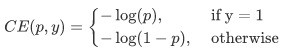
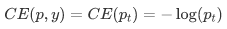
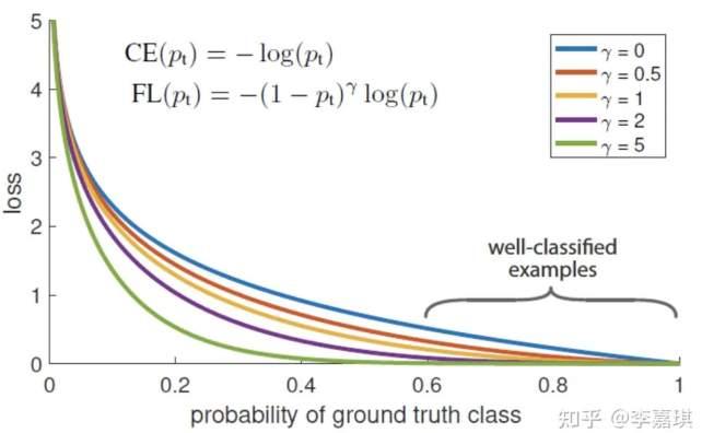
因为是二分类,p表示预测样本属于1的概率(范围为0-1),y表示label,y的取值为{+1,-1}。当真实label是1,也就是y=1时,假如某个样本x预测为1这个类的概率p=0.6,那么损失就是-log(0.6),注意这个损失是大于等于0的。如果p=0.9,那么损失就是-log(0.9),所以p=0.6的损失要大于p=0.9的损失,这很容易理解。这里仅仅以二分类为例,多分类分类以此类推为了方便,用pt代替p,如下公式2:。这里的pt就是前面Figure1中的横坐标。
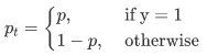
为了表示简便,我们用p_t表示样本属于true class的概率。所以(1)式可以写成:
显然前面的公式3虽然可以控制正负样本的权重,但是没法控制容易分类和难分类样本的权重,于是就有了Focal Loss,这里的γ称作focusing parameter,γ>=0,称为调制系数:
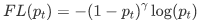
为什么要加上这个调制系数呢?目的是通过减少易分类样本的权重,从而使得模型在训练时更专注于难分类的样本。
通过实验发现,绘制图看如下Figure1,横坐标是pt,纵坐标是loss。CE(pt)表示标准的交叉熵公式,FL(pt)表示focal loss中用到的改进的交叉熵。Figure1中γ=0的蓝色曲线就是标准的交叉熵损失(loss)。
这样就既做到了解决正负样本不平衡,也做到了解决easy与hard样本不平衡的问题。
结论
作者将类别不平衡作为阻碍one-stage方法超过top-performing的two-stage方法的主要原因。为了解决这个问题,作者提出了focal loss,在交叉熵里面用一个调整项,为了将学习专注于hard examples上面,并且降低大量的easy negatives的权值。是同时解决了正负样本不平衡以及区分简单与复杂样本的问题。

我们来看一下,基于MindSpore实现Focal Loss的代码:
import mindspore
import mindspore.common.dtype as mstype
from mindspore.common.tensor import Tensor
from mindspore.common.parameter import Parameter
from mindspore.ops import operations as P
from mindspore.ops import functional as F
from mindspore import nn

class FocalLoss(_Loss):

    def __init__(self, weight=None, gamma=2.0, reduction='mean'):
        super(FocalLoss, self).__init__(reduction=reduction)
        # 校验gamma,这里的γ称作focusing parameter,γ>=0,称为调制系数
        self.gamma = validator.check_value_type("gamma", gamma, [float])
        if weight is not None and not isinstance(weight, Tensor):
            raise TypeError("The type of weight should be Tensor, but got {}.".format(type(weight)))
        self.weight = weight
        # 用到的mindspore算子
        self.expand_dims = P.ExpandDims()
        self.gather_d = P.GatherD()
        self.squeeze = P.Squeeze(axis=1)
        self.tile = P.Tile()
        self.cast = P.Cast()

    def construct(self, predict, target):
        targets = target
        # 对输入进行校验
        _check_ndim(predict.ndim, targets.ndim)
        _check_channel_and_shape(targets.shape[1], predict.shape[1])
        _check_predict_channel(predict.shape[1])

        # 将logits和target的形状更改为num_batch * num_class * num_voxels.
        if predict.ndim > 2:
            predict = predict.view(predict.shape[0], predict.shape[1], -1) # N,C,H,W => N,C,H*W
            targets = targets.view(targets.shape[0], targets.shape[1], -1) # N,1,H,W => N,1,H*W or N,C,H*W
        else:
            predict = self.expand_dims(predict, 2) # N,C => N,C,1
            targets = self.expand_dims(targets, 2) # N,1 => N,1,1 or N,C,1

        # 计算对数概率
        log_probability = nn.LogSoftmax(1)(predict)
        # 只保留每个voxel的地面真值类的对数概率值。
        if target.shape[1] == 1:
            log_probability = self.gather_d(log_probability, 1, self.cast(targets, mindspore.int32))
            log_probability = self.squeeze(log_probability)

        # 得到概率
        probability = F.exp(log_probability)

        if self.weight is not None:
            convert_weight = self.weight[None, :, None]  # C => 1,C,1
            convert_weight = self.tile(convert_weight, (targets.shape[0], 1, targets.shape[2])) # 1,C,1 => N,C,H*W
            if target.shape[1] == 1:
                convert_weight = self.gather_d(convert_weight, 1, self.cast(targets, mindspore.int32))  # selection of the weights  => N,1,H*W
                convert_weight = self.squeeze(convert_weight)  # N,1,H*W => N,H*W
            # 将对数概率乘以它们的权重
            probability = log_probability * convert_weight
        # 计算损失小批量
        weight = F.pows(-probability + 1.0, self.gamma)
        if target.shape[1] == 1:
            loss = (-weight * log_probability).mean(axis=1)  # N
        else:
            loss = (-weight * targets * log_probability).mean(axis=-1)  # N,C

        return self.get_loss(loss)
使用方法如下:
from mindspore.common import dtype as mstype
from mindspore import nn
from mindspore import Tensor

predict = Tensor([[0.8, 1.4], [0.5, 0.9], [1.2, 0.9]], mstype.float32)
target = Tensor([[1], [1], [0]], mstype.int32)
focalloss = nn.FocalLoss(weight=Tensor([1, 2]), gamma=2.0, reduction='mean')
output = focalloss(predict, target)
print(output)

0.33365273
Focal Loss的两个重要性质
1. 当一个样本被分错的时候,pt是很小的,那么调制因子(1-Pt)接近1,损失不被影响;当Pt→1,因子(1-Pt)接近0,那么分的比较好的(well-classified)样本的权值就被调低了。因此调制系数就趋于1,也就是说相比原来的loss是没有什么大的改变的。当pt趋于1的时候(此时分类正确而且是易分类样本),调制系数趋于0,也就是对于总的loss的贡献很小。
2. 当γ=0的时候,focal loss就是传统的交叉熵损失,当γ增加的时候,调制系数也会增加。 专注参数γ平滑地调节了易分样本调低权值的比例。γ增大能增强调制因子的影响,实验发现γ取2最好。直觉上来说,调制因子减少了易分样本的损失贡献,拓宽了样例接收到低损失的范围。当γ一定的时候,比如等于2,一样easy example(pt=0.9)的loss要比标准的交叉熵loss小100+倍,当pt=0.968时,要小1000+倍,但是对于hard example(pt < 0.5),loss最多小了4倍。这样的话hard example的权重相对就提升了很多。这样就增加了那些误分类的重要性Focal Loss的两个性质算是核心,其实就是用一个合适的函数去度量难分类和易分类样本对总的损失的贡献。

MindSpore官方资料:GitHub : https://github.com/mindspore-ai/mindspore
Gitee:https : //gitee.com/mindspore/mindspore
长按下方二维码加入MindSpore项目

本文分享自华为云社区《技术干货 | 基于MindSpore更好的理解Focal Loss》,原文作者:chengxiaoli。

 浙公网安备 33010602011771号