
Rscripts
(一)generating formula
https://stackoverflow.com/questions/4951442/formula-with-dynamic-number-of-variables
for (i in seq_len(factor_number)) {
  for (j in seq(i + 1, factor_number)) {
    linear_model <- lm(Y ~ F1 + F2, list(Y=foo_data_frame$Y,
                                         F1=foo_data_frame[[i]],
                                         F2=foo_data_frame[[j]]))
    # linear_model further analyzing...
  }
}
See ?as.formula, e.g.:
factors <- c("factor1", "factor2")
as.formula(paste("y~", paste(factors, collapse="+")))
# y ~ factor1 + factor2
where factors is a character vector containing the names of the factors you want to use in the model. This you can paste into an lm model, e.g.:
set.seed(0)
y <- rnorm(100)
factor1 <- rep(1:2, each=50)
factor2 <- rep(3:4, 50)
lm(as.formula(paste("y~", paste(factors, collapse="+"))))

# Call:
# lm(formula = as.formula(paste("y~", paste(factors, collapse = "+"))))

# Coefficients:
# (Intercept)      factor1      factor2
#    0.542471    -0.002525    -0.147433
Getting the size of a vector: length(c(1,2,3))
function print
(二)subsetting data in lm
> model4 <- lm(LungCapData[1:10, 1] ~ LungCapData[1:10, 2] + LungCapData[1:10, 3] + LungCapData[1:10, 4] + LungCapData[1:10, 5])
> summary(model4)

Call:
lm(formula = LungCapData[1:10, 1] ~ LungCapData[1:10, 2] + LungCapData[1:10,
    3] + LungCapData[1:10, 4] + LungCapData[1:10, 5])

Residuals:
         1          2          3          4          5          6          7          8          9
 1.006e+00  8.327e-17  1.162e-01  1.773e+00  3.168e-01 -1.162e-01 -1.364e+00 -9.059e-01 -7.653e-01
        10
-6.031e-02

Coefficients:
                         Estimate Std. Error t value Pr(>|t|)
(Intercept)               -4.6843     6.3616  -0.736    0.495
LungCapData[1:10, 2]       0.3493     0.2142   1.630    0.164
LungCapData[1:10, 3]       0.1224     0.1317   0.930    0.395
LungCapData[1:10, 4]yes   -0.6192     1.7090  -0.362    0.732
LungCapData[1:10, 5]male   0.4579     1.2773   0.358    0.735

Residual standard error: 1.229 on 5 degrees of freedom
Multiple R-squared:  0.8242,	Adjusted R-squared:  0.6835
F-statistic: 5.859 on 4 and 5 DF,  p-value: 0.03968

>
> model5 <- lm(LungCapData[1:725, 1] ~ LungCapData[1:725, 2] + LungCapData[1:725, 3] + LungCapData[1:725, 4] + LungCapData[1:725, 5])
> summary(model5)

Call:
lm(formula = LungCapData[1:725, 1] ~ LungCapData[1:725, 2] +
    LungCapData[1:725, 3] + LungCapData[1:725, 4] + LungCapData[1:725,
    5])

Residuals:
    Min      1Q  Median      3Q     Max
-3.2915 -0.7360  0.0184  0.7125  3.0599

Coefficients:
                           Estimate Std. Error t value Pr(>|t|)
(Intercept)               -11.33282    0.47245 -23.987  < 2e-16 ***
LungCapData[1:725, 2]       0.16012    0.01806   8.864  < 2e-16 ***
LungCapData[1:725, 3]       0.26363    0.01009  26.123  < 2e-16 ***
LungCapData[1:725, 4]yes   -0.61774    0.12633  -4.890 1.24e-06 ***
LungCapData[1:725, 5]male   0.38528    0.07991   4.822 1.74e-06 ***
---
Signif. codes:  0 ‘***’ 0.001 ‘**’ 0.01 ‘*’ 0.05 ‘.’ 0.1 ‘ ’ 1

Residual standard error: 1.023 on 720 degrees of freedom
Multiple R-squared:  0.8531,	Adjusted R-squared:  0.8523
F-statistic:  1045 on 4 and 720 DF,  p-value: < 2.2e-16

> model0 <- lm(LungCap ~ Age + Height + Smoke + Gender)
> summary(model0)

Call:
lm(formula = LungCap ~ Age + Height + Smoke + Gender)

Residuals:
    Min      1Q  Median      3Q     Max
-3.2915 -0.7360  0.0184  0.7125  3.0599

Coefficients:
             Estimate Std. Error t value Pr(>|t|)
(Intercept) -11.33282    0.47245 -23.987  < 2e-16 ***
Age           0.16012    0.01806   8.864  < 2e-16 ***
Height        0.26363    0.01009  26.123  < 2e-16 ***
Smokeyes     -0.61774    0.12633  -4.890 1.24e-06 ***
Gendermale    0.38528    0.07991   4.822 1.74e-06 ***
---
Signif. codes:  0 ‘***’ 0.001 ‘**’ 0.01 ‘*’ 0.05 ‘.’ 0.1 ‘ ’ 1

Residual standard error: 1.023 on 720 degrees of freedom
Multiple R-squared:  0.8531,	Adjusted R-squared:  0.8523
F-statistic:  1045 on 4 and 720 DF,  p-value: < 2.2e-16
(三)getting coef, r squared from summary(mod)
http://www.cnblogs.com/howlowl/p/8512222.html
> mod <- lm(LungCap ~ Age)
> mod

Call:
lm(formula = LungCap ~ Age)

Coefficients:
(Intercept)          Age
     1.1469       0.5448

> summary(mod)

Call:
lm(formula = LungCap ~ Age)

Residuals:
    Min      1Q  Median      3Q     Max
-4.7799 -1.0203 -0.0005  0.9789  4.2650

Coefficients:
            Estimate Std. Error t value Pr(>|t|)
(Intercept)  1.14686    0.18353   6.249 7.06e-10 ***
Age          0.54485    0.01416  38.476  < 2e-16 ***
---
Signif. codes:  0 ‘***’ 0.001 ‘**’ 0.01 ‘*’ 0.05 ‘.’ 0.1 ‘ ’ 1

Residual standard error: 1.526 on 723 degrees of freedom
Multiple R-squared:  0.6719,    Adjusted R-squared:  0.6714
F-statistic:  1480 on 1 and 723 DF,  p-value: < 2.2e-16

> attributes(summary(mod))
$names
 [1] "call"          "terms"         "residuals"     "coefficients"  "aliased"       "sigma"
 [7] "df"            "r.squared"     "adj.r.squared" "fstatistic"    "cov.unscaled"

$class
[1] "summary.lm"

> summary(mod)$r.squared
[1] 0.6718669
> summary(mod)$adj.r.squared
[1] 0.6714131
> summary(mod)$coefficients[, 4]
  (Intercept)           Age
 7.056380e-10 4.077172e-177
> summary(mod)$coefficients[,1:4]
             Estimate Std. Error   t value      Pr(>|t|)
(Intercept) 1.1468578 0.18352850  6.248936  7.056380e-10
Age         0.5448484 0.01416087 38.475634 4.077172e-177
> class(summary(mod))
[1] "summary.lm"
> class(summary(mod)$coefficients)
[1] "matrix"
> class(summary(mod)$coefficients[,4])
[1] "numeric"
> class(summary(mod)$coefficients[,1:4])
[1] "matrix"
>
> summary(mod)$coefficients[, 4]["(Intercept)"]
(Intercept)
7.05638e-10
> summary(mod)$coefficients[, 4]["Age"]
          Age
4.077172e-177
>
> summary(mod)$coefficients[, 4][1]
(Intercept)
7.05638e-10
> summary(mod)$coefficients[, 4][2]
          Age
4.077172e-177
> summary(mod)$coefficients[, 4][3]
<NA>
  NA
(四)append values to vector in r
Here are several ways to do it. All of them are discouraged. Appending to an object in a for loop causes the entire object to be copied on every iteration, which causes a lot of people to say "R is slow", or "R loops should be avoided".
# one way
for (i in 1:length(values))
  vector[i] <- values[i]
# another way
for (i in 1:length(values))
  vector <- c(vector, values[i])
# yet another way?!?
for (v in values)
  vector <- c(vector, v)
# ... more ways
help("append") would have answered your question and saved the time it took you to write this question (but would have caused you to develop bad habits). ;-)
Note that vector <- c() isn't an empty vector; it's NULL. If you want an empty character vector, use vector <- character().
Also note, as BrodieG pointed out in the comments: if you absolutely must use a for loop, then at least pre-allocate the entire vector before the loop. This will be much faster than appending for larger vectors.
set.seed(21)
values <- sample(letters, 1e4, TRUE)
vector <- character(0)
# slow
system.time( for (i in 1:length(values)) vector[i] <- values[i] )
#   user  system elapsed
#  0.340   0.000   0.343
vector <- character(length(values))
# fast(er)
system.time( for (i in 1:length(values)) vector[i] <- values[i] )
#   user  system elapsed
#  0.024   0.000   0.023
-------------------------------------------------
> c(1, 7:9)
[1] 1 7 8 9
> c(1:5, 10.5, "next")
[1] "1"    "2"    "3"    "4"    "5"    "10.5" "next"
> x = 1:4
> x
[1] 1 2 3 4
> names(x) = letters[1:4]
> x
a b c d
1 2 3 4
> letters
 [1] "a" "b" "c" "d" "e" "f" "g" "h" "i" "j" "k" "l" "m" "n" "o" "p" "q" "r" "s" "t" "u" "v" "w" "x" "y" "z"
> c(x)
a b c d
1 2 3 4
> as.vector(x)
[1] 1 2 3 4
> dim(x) = c(2,2)
> x
     [,1] [,2]
[1,]    1    3
[2,]    2    4
> x
     [,1] [,2]
[1,]    1    3
[2,]    2    4
> c(x)
[1] 1 2 3 4
> as.vector(x)
[1] 1 2 3 4
> #append to a list
> ll = list(A =1, c = "C")
> ll
$A
[1] 1

$c
[1] "C"

> c(ll, d = list(1:3))
$A
[1] 1

$c
[1] "C"

$d
[1] 1 2 3

> c(ll, d=1:3)
$A
[1] 1

$c
[1] "C"

$d1
[1] 1

$d2
[1] 2

$d3
[1] 3

> c(ll, as.list(c(d=1:3)))
$A
[1] 1

$c
[1] "C"

$d1
[1] 1

$d2
[1] 2

$d3
[1] 3

>
> c(list(A = c(B = 1)), recursive= T)
A.B
  1
(四)pvcm: panel data with variable coefficients for individuals

pvcm (in plm package):
> zw <- pvcm(log(gsp) ~ log(pcap) + log(pc) + log(emp) + unemp, data = Produc, model = "within")
> summary(zw)
Oneway (individual) effect No-pooling model

Call:
pvcm(formula = log(gsp) ~ log(pcap) + log(pc) + log(emp) + unemp,
    data = Produc, model = "within")

Balanced Panel: n = 48, T = 17, N = 816

Residuals:
      Min.    1st Qu.     Median       Mean    3rd Qu.       Max.
-0.0828079 -0.0118150  0.0004247  0.0000000  0.0126479  0.1189647

Coefficients:
  (Intercept)       log(pcap)          log(pc)            log(emp)            unemp
 Min.   :-3.708   Min.   :-1.4426   Min.   :-0.52365   Min.   :-0.02584   Min.   :-0.027617
 1st Qu.: 1.229   1st Qu.:-0.5065   1st Qu.:-0.02584   1st Qu.: 0.61569   1st Qu.:-0.012080
 Median : 2.733   Median :-0.1086   Median : 0.23335   Median : 0.87256   Median :-0.003905
 Mean   : 2.672   Mean   :-0.1049   Mean   : 0.21825   Mean   : 0.93348   Mean   :-0.003722
 3rd Qu.: 4.214   3rd Qu.: 0.2682   3rd Qu.: 0.41768   3rd Qu.: 1.25307   3rd Qu.: 0.002948
 Max.   : 9.338   Max.   : 1.0312   Max.   : 1.23217   Max.   : 2.10582   Max.   : 0.029017

Total Sum of Squares: 19352
Residual Sum of Squares: 0.33009
Multiple R-Squared: 0.99998
> #residual sum of squares RSS 残差平方和
> sum(zw$residuals^2)
[1] 0.3300925
(五)find xx percentile for F distribution
If V 1 and V 2 are two independent random variables having the Chi-Squared distribution with m1 and m2 degrees of freedom respectively, then the following quantity follows an F distribution with m1 numerator degrees of freedom and m2 denominator degrees of freedom, i.e., (m1,m2) degrees of freedom.
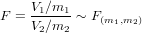
Here is a graph of the F distribution with (5, 2) degrees of freedom.
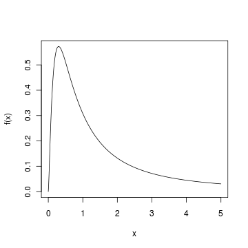
Find the 95th percentile of the F distribution with (5, 2) degrees of freedom.
We apply the quantile function qf of the F distribution against the decimal value 0.95.
(六)vector and list
> #vector: all elements must be the same type
> name = c("Mike", "Lucy", "Jack")
> age = c(18, 19, 20)
>
> name[c(2, 3)]
[1] "Lucy" "Jack"
> #array&matrix: vector with attributes(nrow and ncol)
> x = matrix(c(1,2,3,4), nrow=2, ncol=2)
> x
     [,1] [,2]
[1,]    1    3
[2,]    2    4
> y = list(name="Mike", gender="M", company="ProgramCreek")
> y
$name
[1] "Mike"

$gender
[1] "M"

$company
[1] "ProgramCreek"

> student = c(T,F,T)
> df = data.frame(name, age, student)
> df
  name age student
1 Mike  18    TRUE
2 Lucy  19   FALSE
> #vector: all elements must be the same type
> name = c("Mike", "Lucy", "Jack")
> age = c(18, 19, 20)
>
> name[c(2, 3)]
[1] "Lucy" "Jack"
> #array&matrix: vector with attributes(nrow and ncol)
> x = matrix(c(1,2,3,4), nrow=2, ncol=2)
> x
     [,1] [,2]
[1,]    1    3
[2,]    2    4
> y = list(name="Mike", gender="M", company="ProgramCreek")
> y
$name
[1] "Mike"

$gender
[1] "M"

$company
[1] "ProgramCreek"

> student = c(T,F,T)
> df = data.frame(name, age, student)
> df
  name age student
1 Mike  18    TRUE
2 Lucy  19   FALSE
3 Jack  20    TRUE
>
>
>
> cells = c(1,26,24,68)
> rnames = c("R1", "R2")
> cnames = c("C1", "C2")
> mymatrix = matrix(cells, nrow=2, ncol=2, byrow=T, dimnames = list(rnames, cnames))
> mymatrix
   C1 C2
R1  1 26
R2 24 68
>
> #data frames
> d = c(1,2,3,4)
> e = c(T,T,T,F)
> f = c("red", "white", "red", NA)
> mydata = data.frame(d,e,f)
> names(mydata) = c("ID", "Passed", "Color")
> mydata
  ID Passed Color
1  1   TRUE   red
2  2   TRUE white
3  3   TRUE   red
4  4  FALSE  <NA>
>
> #list
> a <- c(1,2,5.3,6,-2,4)
> w = list(name = "Fred", mynumbers = a, mymatrix = mymatrix, age = 5.3)
> w
$name
[1] "Fred"

$mynumbers
[1]  1.0  2.0  5.3  6.0 -2.0  4.0

$mymatrix
   C1 C2
R1  1 26
R2 24 68

$age
[1] 5.3

> v = c(y, w)
> v
$name
[1] "Mike"

$gender
[1] "M"

$company
[1] "ProgramCreek"

$name
[1] "Fred"

$mynumbers
[1]  1.0  2.0  5.3  6.0 -2.0  4.0

$mymatrix
   C1 C2
R1  1 26
R2 24 68

$age
[1] 5.3

> v = c(w, y)
> v
$name
[1] "Fred"

$mynumbers
[1]  1.0  2.0  5.3  6.0 -2.0  4.0

$mymatrix
   C1 C2
R1  1 26
R2 24 68

$age
[1] 5.3

$name
[1] "Mike"

$gender
[1] "M"

$company
[1] "ProgramCreek"

> vv = list(w, y)
> vv
[[1]]
[[1]]$name
[1] "Fred"

[[1]]$mynumbers
[1]  1.0  2.0  5.3  6.0 -2.0  4.0

[[1]]$mymatrix
   C1 C2
R1  1 26
R2 24 68

[[1]]$age
[1] 5.3


[[2]]
[[2]]$name
[1] "Mike"

[[2]]$gender
[1] "M"

[[2]]$company
[1] "ProgramCreek"


> vv[[2]]
$name
[1] "Mike"

$gender
[1] "M"

$company
[1] "ProgramCreek"

> vv[["name"]]
NULL
> vv[2]
[[1]]
[[1]]$name
[1] "Mike"

[[1]]$gender
[1] "M"

[[1]]$company
[1] "ProgramCreek"


>
> #factors
> gender = c(rep("male",20), rep("female",30))
> summary(gender)
   Length     Class      Mode
       50 character character
> gender = factor(gender)
> summary(gender)
female   male
    30     20
>
(七)define functions
myfunction <- function(arg1, arg2, ... ){
statements
return(object)
}

 浙公网安备 33010602011771号