
R_MarinStats_Notes3
5.1 simple linear regression in r
> plot(Age, LungCap, main="Scatterplot")
> cor(Age, LungCap)
[1] 0.8196749
>
> ?lm
> mod = lm(LungCap ~ Age)
> summary(mod)

Call:
lm(formula = LungCap ~ Age)

Residuals:
    Min      1Q  Median      3Q     Max
-4.7799 -1.0203 -0.0005  0.9789  4.2650

Coefficients:
            Estimate Std. Error t value Pr(>|t|)
(Intercept)  1.14686    0.18353   6.249 7.06e-10 ***
Age          0.54485    0.01416  38.476  < 2e-16 ***
---
Signif. codes:  0 ‘***’ 0.001 ‘**’ 0.01 ‘*’ 0.05 ‘.’ 0.1 ‘ ’ 1

Residual standard error: 1.526 on 723 degrees of freedom
Multiple R-squared:  0.6719,	Adjusted R-squared:  0.6714
F-statistic:  1480 on 1 and 723 DF,  p-value: < 2.2e-16

> attributes(mod)
$names
 [1] "coefficients"  "residuals"     "effects"       "rank"          "fitted.values" "assign"
 [7] "qr"            "df.residual"   "xlevels"       "call"          "terms"         "model"

$class
[1] "lm"

> mod$coefficients
(Intercept)         Age
  1.1468578   0.5448484
> coef(mod)
(Intercept)         Age
  1.1468578   0.5448484
> plot(Age, LungCap, main="Scatterplot")
> abline(mod, col=2, lwd=3)
>
> confint(mod)
                2.5 %    97.5 %
(Intercept) 0.7865454 1.5071702
Age         0.5170471 0.5726497
> confint(mod, level=0.99)
0.5 % 99.5 %
(Intercept) 0.6728686 1.6208470
Age 0.5082759 0.5814209

> summary(mod)

Call:
lm(formula = LungCap ~ Age)

Residuals:
    Min      1Q  Median      3Q     Max
-4.7799 -1.0203 -0.0005  0.9789  4.2650

Coefficients:
            Estimate Std. Error t value Pr(>|t|)
(Intercept)  1.14686    0.18353   6.249 7.06e-10 ***
Age          0.54485    0.01416  38.476  < 2e-16 ***
---
Signif. codes:  0 ‘***’ 0.001 ‘**’ 0.01 ‘*’ 0.05 ‘.’ 0.1 ‘ ’ 1

Residual standard error: 1.526 on 723 degrees of freedom
Multiple R-squared:  0.6719,	Adjusted R-squared:  0.6714
F-statistic:  1480 on 1 and 723 DF,  p-value: < 2.2e-16

> anova(mod)
Analysis of Variance Table

Response: LungCap
           Df Sum Sq Mean Sq F value    Pr(>F)
Age         1 3447.0  3447.0  1480.4 < 2.2e-16 ***
Residuals 723 1683.5     2.3
---
Signif. codes:  0 ‘***’ 0.001 ‘**’ 0.01 ‘*’ 0.05 ‘.’ 0.1 ‘ ’ 1
>
> sqrt(2.3)
[1] 1.516575
> # 1.516575 is equal to 1.526
MORE INFO:3
https://stackoverflow.com/questions/5587676/pull-out-p-values-and-r-squared-from-a-linear-regression
Notice that summary(fit) generates an object with all the information you need. The beta, se, t and p vectors are stored in it. Get the p-values by selecting the 4th column of the coefficients matrix (stored in the summary object):
summary(fit)$coefficients[,4]
summary(fit)$r.squared
Try str(summary(fit)) to see all the info that this object contains.
> mod <- lm(LungCap ~ Age)
> mod

Call:
lm(formula = LungCap ~ Age)

Coefficients:
(Intercept)          Age
     1.1469       0.5448

> summary(mod)

Call:
lm(formula = LungCap ~ Age)

Residuals:
    Min      1Q  Median      3Q     Max
-4.7799 -1.0203 -0.0005  0.9789  4.2650

Coefficients:
            Estimate Std. Error t value Pr(>|t|)
(Intercept)  1.14686    0.18353   6.249 7.06e-10 ***
Age          0.54485    0.01416  38.476  < 2e-16 ***
---
Signif. codes:  0 ‘***’ 0.001 ‘**’ 0.01 ‘*’ 0.05 ‘.’ 0.1 ‘ ’ 1

Residual standard error: 1.526 on 723 degrees of freedom
Multiple R-squared:  0.6719,	Adjusted R-squared:  0.6714
F-statistic:  1480 on 1 and 723 DF,  p-value: < 2.2e-16

> attributes(summary(mod))
$names
 [1] "call"          "terms"         "residuals"     "coefficients"  "aliased"       "sigma"
 [7] "df"            "r.squared"     "adj.r.squared" "fstatistic"    "cov.unscaled"

$class
[1] "summary.lm"

> summary(mod)$r.squared
[1] 0.6718669
> summary(mod)$adj.r.squared
[1] 0.6714131
> summary(mod)$coefficients[, 4]
  (Intercept)           Age
 7.056380e-10 4.077172e-177
> summary(mod)$coefficients[,1:4]
             Estimate Std. Error   t value      Pr(>|t|)
(Intercept) 1.1468578 0.18352850  6.248936  7.056380e-10
Age         0.5448484 0.01416087 38.475634 4.077172e-177
> class(summary(mod))
[1] "summary.lm"
> class(summary(mod)$coefficients)
[1] "matrix"
> class(summary(mod)$coefficients[,4])
[1] "numeric"
> class(summary(mod)$coefficients[,1:4])
[1] "matrix"
>
> summary(mod)$coefficients[, 4]["(Intercept)"]
(Intercept)
7.05638e-10
> summary(mod)$coefficients[, 4]["Age"]
          Age
4.077172e-177
>
> summary(mod)$coefficients[, 4][1]
(Intercept)
7.05638e-10
> summary(mod)$coefficients[, 4][2]
          Age
4.077172e-177
> summary(mod)$coefficients[, 4][3]
<NA>
  NA
Interpreting output from anova() when using lm() as input:
https://stats.stackexchange.com/questions/115304/interpreting-output-from-anova-when-using-lm-as-input
https://stats.stackexchange.com/questions/5135/interpretation-of-rs-lm-output
The anova() function call returns an ANOVA table. You can use it to get an ANOVA table any time you want one. Thus, the question becomes, 'why might I want an ANOVA table when I can just get tt-tests of my variables with standard output (i.e., the summary.lm() command)?'
First of all, you may be perfectly satisfied with the summary output, and that's fine. However, the ANOVA table may offer some advantages. First, if you have a categorical / factor variable with more than two levels, the summary output is hard to interpret. It will give you tests of individual levels against the reference level, but won't give you a test of the factor as a whole. Consider:
set.seed(8867)                           # this makes the example exactly reproducible
y     = c(rnorm(10, mean=0,   sd=1),
          rnorm(10, mean=-.5, sd=1),
          rnorm(10, mean=.5,  sd=1) )
g     = rep(c("A", "B", "C"), each=10)
model = lm(y~g)
summary(model)
# ...
# Residuals:
#      Min       1Q   Median       3Q      Max
# -2.59080 -0.54685  0.04124  0.79890  2.56064
#
# Coefficients:
#             Estimate Std. Error t value Pr(>|t|)
# (Intercept)  -0.4440     0.3855  -1.152    0.260
# gB           -0.9016     0.5452  -1.654    0.110
# gC            0.6729     0.5452   1.234    0.228
#
# Residual standard error: 1.219 on 27 degrees of freedom
# Multiple R-squared:  0.2372,  Adjusted R-squared:  0.1807
# F-statistic: 4.199 on 2 and 27 DF,  p-value: 0.02583
anova(model)
# Analysis of Variance Table
#
# Response: y
#           Df Sum Sq Mean Sq F value  Pr(>F)
# g          2 12.484  6.2418   4.199 0.02583 *
# Residuals 27 40.135  1.4865
Another reason you might prefer to look at an ANOVA table is that it allows you to use information about the possible associations between your independent variables and your dependent variable that gets thrown away by the tt-tests in the summary output. Consider your own example, you may notice that the pp-values from the two don't match (e.g., for v1, the pp-value in the summary output is 0.93732, but in the ANOVA table it's 0.982400). The reason is that your variables are not perfectly uncorrelated:
cor(my_data)
#                   v1          v2         v3    response
# v1        1.00000000 -0.23760679 -0.1312995 -0.00357923
# v2       -0.23760679  1.00000000 -0.2358402  0.06069167
# v3       -0.13129952 -0.23584024  1.0000000  0.32818751
# response -0.00357923  0.06069167  0.3281875  1.00000000
The result of this is that there are sums of squares that could be attributed to more than one of the variables. The tt-tests are equivalent to 'type III' tests of the sums of squares, but other tests are possible. The default ANOVA table uses 'type I' sums of squares, which can allow you to make more precise--and more powerful--tests of your hypotheses.
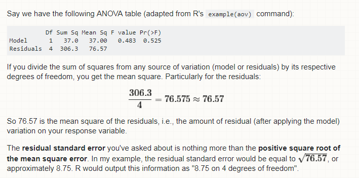
总离差平方和:SST(Sum of Squares for total) = TSS(total sum of squares)
SSE+SSR=SST RSS+ESS=TSS
> plot(mod)
Hit <Return> to see next plot:
Hit <Return> to see next plot:
Hit <Return> to see next plot:
Hit <Return> to see next plot:
> par(mfrow=c(2,2))
> plot(mod)
> par(mfrow=c(1,1))
> plot(mod)
Hit <Return> to see next plot:
Hit <Return> to see next plot:
Hit <Return> to see next plot:
Hit <Return> to see next plot:
5.3 multiple linear regression
> model1 <- lm(LungCap ~ Age+Height)
> summary(model1)

Call:
lm(formula = LungCap ~ Age + Height)

Residuals:
    Min      1Q  Median      3Q     Max
-3.4080 -0.7097 -0.0078  0.7167  3.1679

Coefficients:
              Estimate Std. Error t value Pr(>|t|)
(Intercept) -11.747065   0.476899 -24.632  < 2e-16 ***
Age           0.126368   0.017851   7.079 3.45e-12 ***
Height        0.278432   0.009926  28.051  < 2e-16 ***
---
Signif. codes:  0 ‘***’ 0.001 ‘**’ 0.01 ‘*’ 0.05 ‘.’ 0.1 ‘ ’ 1

Residual standard error: 1.056 on 722 degrees of freedom
Multiple R-squared:  0.843,	Adjusted R-squared:  0.8425
F-statistic:  1938 on 2 and 722 DF,  p-value: < 2.2e-16

> anova(model1)
Analysis of Variance Table

Response: LungCap
           Df Sum Sq Mean Sq F value    Pr(>F)
Age         1 3447.0  3447.0 3089.42 < 2.2e-16 ***
Height      1  877.9   877.9  786.84 < 2.2e-16 ***
Residuals 722  805.6     1.1
---
Signif. codes:  0 ‘***’ 0.001 ‘**’ 0.01 ‘*’ 0.05 ‘.’ 0.1 ‘ ’ 1
> cor(Age, Height, method="pearson")
[1] 0.8357368
> confint(model1, level=0.95)
                   2.5 %      97.5 %
(Intercept) -12.68333877 -10.8107918
Age           0.09132215   0.1614142
Height        0.25894454   0.2979192
> model2<- lm(LungCap ~ Age+Height+Smoke+Gender+Caesarean)
> summary(model2)

Call:
lm(formula = LungCap ~ Age + Height + Smoke + Gender + Caesarean)

Residuals:
    Min      1Q  Median      3Q     Max
-3.3388 -0.7200  0.0444  0.7093  3.0172

Coefficients:
              Estimate Std. Error t value Pr(>|t|)
(Intercept)  -11.32249    0.47097 -24.041  < 2e-16 ***
Age            0.16053    0.01801   8.915  < 2e-16 ***
Height         0.26411    0.01006  26.248  < 2e-16 ***
Smokeyes      -0.60956    0.12598  -4.839 1.60e-06 ***
Gendermale     0.38701    0.07966   4.858 1.45e-06 ***
Caesareanyes  -0.21422    0.09074  -2.361   0.0185 *
---
Signif. codes:  0 ‘***’ 0.001 ‘**’ 0.01 ‘*’ 0.05 ‘.’ 0.1 ‘ ’ 1

Residual standard error: 1.02 on 719 degrees of freedom
Multiple R-squared:  0.8542,	Adjusted R-squared:  0.8532
F-statistic: 842.8 on 5 and 719 DF,  p-value: < 2.2e-16

> plot(model2)
Hit <Return> to see next plot:
Hit <Return> to see next plot:
Hit <Return> to see next plot:
Hit <Return> to see next plot:
5.4 converting a numeric variable to a categorical variable in r
useful for making some cross-tabulations for a variable, or fitting a regression model when the linearity assumption is not valid for the variable
> ?cut
> #A <=50, B(50,55], C(55,60], D(60,65], E(65,70], F>70
> CatHeight <- cut(Height, breaks = c(0,50,55,60,65,70,100), labels=c("A","B","C","D","E","F"))
> Height[1:10]
 [1] 62.1 74.7 69.7 71.0 56.9 58.7 63.3 70.4 70.5 59.2
> CatHeight[1:10]
 [1] D F E F C C D F F C
Levels: A B C D E F
> #right = False [a, b)
> CatHeight <- cut(Height, breaks = c(0,50,55,60,65,70,100), labels=c("A","B","C","D","E","F"), right = F)
> Height[1:10]
 [1] 62.1 74.7 69.7 71.0 56.9 58.7 63.3 70.4 70.5 59.2
> CatHeight[1:10]
 [1] D F E F C C D F F C
Levels: A B C D E F
> CatHeight <- cut(Height, breaks = c(0,50,55,60,65,70,100), right = F)
> CatHeight[1:10]
 [1] [60,65)  [70,100) [65,70)  [70,100) [55,60)  [55,60)  [60,65)  [70,100) [70,100) [55,60)
Levels: [0,50) [50,55) [55,60) [60,65) [65,70) [70,100)
> CatHeight <- cut(Height, breaks = 4, right = F)
> CatHeight[1:10]
 [1] [54.4,63.5) [72.7,81.8) [63.5,72.7) [63.5,72.7) [54.4,63.5) [54.4,63.5) [54.4,63.5) [63.5,72.7)
 [9] [63.5,72.7) [54.4,63.5)
Levels: [45.3,54.4) [54.4,63.5) [63.5,72.7) [72.7,81.8)
5.5 dummy variable or indicator variables in r
> CatHeight <- cut(Height, breaks = c(0,50,55,60,65,70,100), labels=c("A","B","C","D","E","F"), right = F)
> CatHeight[1:10]
 [1] D F E F C C D F F C
Levels: A B C D E F
> levels(Smoke)
[1] "no"  "yes"
> #2 levels require 1 indicator variable to represent smoking status
>
> levels(CatHeight)
[1] "A" "B" "C" "D" "E" "F"
> mean(LungCap[CatHeight == "A"])
[1] 2.148611
> mean(LungCap[CatHeight == "B"])
[1] 3.65464
> mean(LungCap[CatHeight == "C"])
[1] 5.396983
> mean(LungCap[CatHeight == "D"])
[1] 7.170552
> mean(LungCap[CatHeight == "E"])
[1] 8.692063
> mean(LungCap[CatHeight == "F"])
[1] 10.80278
> mod <- lm(LungCap ~ CatHeight)
> summary(mod)

Call:
lm(formula = LungCap ~ CatHeight)

Residuals:
    Min      1Q  Median      3Q     Max
-3.9671 -0.7720 -0.0456  0.7972  3.8722

Coefficients:
            Estimate Std. Error t value Pr(>|t|)
(Intercept)   2.1486     0.2929   7.336 5.97e-13 ***
CatHeightB    1.5060     0.3416   4.409 1.20e-05 ***
CatHeightC    3.2484     0.3148  10.319  < 2e-16 ***
CatHeightD    5.0219     0.3086  16.271  < 2e-16 ***
CatHeightE    6.5435     0.3065  21.347  < 2e-16 ***
CatHeightF    8.6542     0.3065  28.233  < 2e-16 ***
---
Signif. codes:  0 ‘***’ 0.001 ‘**’ 0.01 ‘*’ 0.05 ‘.’ 0.1 ‘ ’ 1

Residual standard error: 1.243 on 719 degrees of freedom
Multiple R-squared:  0.7836,	Adjusted R-squared:  0.7821
F-statistic: 520.7 on 5 and 719 DF,  p-value: < 2.2e-16
5.6 Changing baseline(Reference) Category for a Categorical Variable in a linear regression model in r
By default, the category that R chooses to be the reference or baseline, is the first category that appears alphabetically or numerically. ('no' in this case)
> ?relevel
> mod1 <- lm(LungCap ~ Age + Smoke)
> summary(mod1)

Call:
lm(formula = LungCap ~ Age + Smoke)

Residuals:
    Min      1Q  Median      3Q     Max
-4.8559 -1.0289 -0.0363  1.0083  4.1995

Coefficients:
            Estimate Std. Error t value Pr(>|t|)
(Intercept)  1.08572    0.18299   5.933 4.61e-09 ***
Age          0.55540    0.01438  38.628  < 2e-16 ***
Smokeyes    -0.64859    0.18676  -3.473 0.000546 ***
---
Signif. codes:  0 ‘***’ 0.001 ‘**’ 0.01 ‘*’ 0.05 ‘.’ 0.1 ‘ ’ 1

Residual standard error: 1.514 on 722 degrees of freedom
Multiple R-squared:  0.6773,	Adjusted R-squared:  0.6764
F-statistic: 757.5 on 2 and 722 DF,  p-value: < 2.2e-16

> table(Smoke)
Smoke
 no yes
648  77
>
> Smoke <- relevel(Smoke, ref="yes")
> table(Smoke)
Smoke
yes  no
 77 648
> mod2 <- lm(LungCap ~ Age + Smoke)
> summary(mod2)

Call:
lm(formula = LungCap ~ Age + Smoke)

Residuals:
    Min      1Q  Median      3Q     Max
-4.8559 -1.0289 -0.0363  1.0083  4.1995

Coefficients:
            Estimate Std. Error t value Pr(>|t|)
(Intercept)  0.43714    0.27375   1.597 0.110740
Age          0.55540    0.01438  38.628  < 2e-16 ***
Smokeno      0.64859    0.18676   3.473 0.000546 ***
---
Signif. codes:  0 ‘***’ 0.001 ‘**’ 0.01 ‘*’ 0.05 ‘.’ 0.1 ‘ ’ 1

Residual standard error: 1.514 on 722 degrees of freedom
Multiple R-squared:  0.6773,	Adjusted R-squared:  0.6764
F-statistic: 757.5 on 2 and 722 DF,  p-value: < 2.2e-16
5.7 categorical variable into regression model in r
assumes there is no interaction between smoking and age
> model1 <- lm(LungCap ~ Age + Smoke)
> summary(model1)

Call:
lm(formula = LungCap ~ Age + Smoke)

Residuals:
    Min      1Q  Median      3Q     Max
-4.8559 -1.0289 -0.0363  1.0083  4.1995

Coefficients:
            Estimate Std. Error t value Pr(>|t|)
(Intercept)  1.08572    0.18299   5.933 4.61e-09 ***
Age          0.55540    0.01438  38.628  < 2e-16 ***
Smokeyes    -0.64859    0.18676  -3.473 0.000546 ***
---
Signif. codes:  0 ‘***’ 0.001 ‘**’ 0.01 ‘*’ 0.05 ‘.’ 0.1 ‘ ’ 1

Residual standard error: 1.514 on 722 degrees of freedom
Multiple R-squared:  0.6773,	Adjusted R-squared:  0.6764
F-statistic: 757.5 on 2 and 722 DF,  p-value: < 2.2e-16

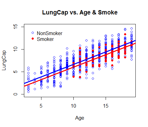
> plot(Age[Smoke=="no"], LungCap[Smoke=="no"], col="blue", ylim=c(0,15), xlab="Age", ylab="LungCap", main="LungCap vs. Age & Smoke")
> points(Age[Smoke=="yes"], LungCap[Smoke=="yes"], col="red", pch=16)
> legend(3, 15, legend = c("NonSmoker", "Smoker"), col=c("blue", "red"), pch=c(1,16), bty="n")
>
> abline(a=1.08, b=0.555, col="blue", lwd=3)
> abline(a=1.08-0.64859, b=0.555, col="red", lwd=3)
5.8 another example of including a categorical variable into a regression model in r
> levels(CatHeight)
[1] "A" "B" "C" "D" "E" "F"
> model2 <- lm(LungCap ~ Age + CatHeight)
> summary(model2)

Call:
lm(formula = LungCap ~ Age + CatHeight)

Residuals:
    Min      1Q  Median      3Q     Max
-3.8492 -0.7711  0.0037  0.7449  3.4230

Coefficients:
            Estimate Std. Error t value Pr(>|t|)
(Intercept)  0.99913    0.29371   3.402 0.000707 ***
Age          0.19705    0.01868  10.546  < 2e-16 ***
CatHeightB   1.48107    0.31808   4.656 3.83e-06 ***
CatHeightC   2.67193    0.29819   8.961  < 2e-16 ***
CatHeightD   3.92646    0.30560  12.848  < 2e-16 ***
CatHeightE   5.01342    0.32019  15.658  < 2e-16 ***
CatHeightF   6.58093    0.34658  18.988  < 2e-16 ***
---
Signif. codes:  0 ‘***’ 0.001 ‘**’ 0.01 ‘*’ 0.05 ‘.’ 0.1 ‘ ’ 1

Residual standard error: 1.157 on 718 degrees of freedom
Multiple R-squared:  0.8126,	Adjusted R-squared:  0.811
F-statistic: 518.9 on 6 and 718 DF,  p-value: < 2.2e-16


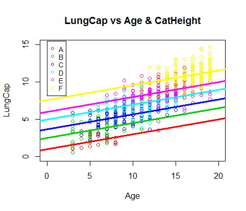
> plot(Age[CatHeight=="A"], LungCap[CatHeight=="A"], col=2, ylim = c(0,15), xlim=c(0,20), xlab="Age", ylab = "LungCap", main = "LungCap vs Age & CatHeight")
> points(Age[CatHeight=="B"], LungCap[CatHeight=="B"], col=3)
> points(Age[CatHeight=="C"], LungCap[CatHeight=="C"], col=4)
> points(Age[CatHeight=="D"], LungCap[CatHeight=="D"], col=5)
> points(Age[CatHeight=="E"], LungCap[CatHeight=="E"], col=6)
> points(Age[CatHeight=="F"], LungCap[CatHeight=="F"], col=7)
>
> legend(0, 15.5, legend=c("A","B","C","D","E","F"), col=c(2:7), pch=1, cex=0.8)
>
> abline(a=0.98, b=0.20, col =2, lwd=3)
> abline(a=2.46, b=0.20, col =3, lwd=3)
> abline(a=3.67, b=0.20, col =4, lwd=3)
> abline(a=4.92, b=0.20, col =5, lwd=3)
> abline(a=5.99, b=0.20, col =6, lwd=3)
> abline(a=7.52, b=0.20, col =7, lwd=3)
5.9 multiple linear regression with interaction in R
If x1 and x2 interact, this means that the effect of x1 on y depends on the value of x2, and vice versa
(the effect of age is modified by smoking)
> model1 <- lm(LungCap ~ Age * Smoke)
> coef(model1)
 (Intercept)          Age     Smokeyes Age:Smokeyes
  1.05157244   0.55823350   0.22601390  -0.05970463
> model1 <- lm(LungCap ~ Age + Smoke + Age:Smoke)
> summary(model1)

Call:
lm(formula = LungCap ~ Age + Smoke + Age:Smoke)

Residuals:
    Min      1Q  Median      3Q     Max
-4.8586 -1.0174 -0.0251  1.0004  4.1996

Coefficients:
             Estimate Std. Error t value Pr(>|t|)
(Intercept)   1.05157    0.18706   5.622  2.7e-08 ***
Age           0.55823    0.01473  37.885  < 2e-16 ***
Smokeyes      0.22601    1.00755   0.224    0.823
Age:Smokeyes -0.05970    0.06759  -0.883    0.377
---
Signif. codes:  0 ‘***’ 0.001 ‘**’ 0.01 ‘*’ 0.05 ‘.’ 0.1 ‘ ’ 1

Residual standard error: 1.515 on 721 degrees of freedom
Multiple R-squared:  0.6776,	Adjusted R-squared:  0.6763
F-statistic: 505.1 on 3 and 721 DF,  p-value: < 2.2e-16
Age:Smokeyes is not significant, the interaction should not be included in the model
5.10 interaction between factors in a linear regression model
5.11 comparing models using the partial F-test in R
partial F-test is used in model building and variable selection to help decide if a variable or term can be removed from a model without making the model significantly worse (does it result in a statistically significant increase in the sum of the squared errors a.k.a. residual sum of squares?)
Full model, reduced modeld
partial F-test is used to test nested model
H0: no significant difference in sse of full and reduced models
H1: full model has a significantly lower sse than the reduced model
> Full.Model <- lm(LungCap ~ Age + I(Age^2))
> Reduced.Model <- lm(LungCap ~ Age)
> summary(Full.Model)

Call:
lm(formula = LungCap ~ Age + I(Age^2))

Residuals:
    Min      1Q  Median      3Q     Max
-4.8446 -1.0150 -0.0212  1.0442  4.1942

Coefficients:
             Estimate Std. Error t value Pr(>|t|)
(Intercept)  0.610275   0.433197   1.409    0.159
Age          0.647707   0.076549   8.461   <2e-16 ***
I(Age^2)    -0.004354   0.003184  -1.367    0.172
---
Signif. codes:  0 ‘***’ 0.001 ‘**’ 0.01 ‘*’ 0.05 ‘.’ 0.1 ‘ ’ 1

Residual standard error: 1.525 on 722 degrees of freedom
Multiple R-squared:  0.6727,	Adjusted R-squared:  0.6718
F-statistic:   742 on 2 and 722 DF,  p-value: < 2.2e-16

> summary(Reduced.Model)

Call:
lm(formula = LungCap ~ Age)

Residuals:
    Min      1Q  Median      3Q     Max
-4.7799 -1.0203 -0.0005  0.9789  4.2650

Coefficients:
            Estimate Std. Error t value Pr(>|t|)
(Intercept)  1.14686    0.18353   6.249 7.06e-10 ***
Age          0.54485    0.01416  38.476  < 2e-16 ***
---
Signif. codes:  0 ‘***’ 0.001 ‘**’ 0.01 ‘*’ 0.05 ‘.’ 0.1 ‘ ’ 1

Residual standard error: 1.526 on 723 degrees of freedom
Multiple R-squared:  0.6719,	Adjusted R-squared:  0.6714
F-statistic:  1480 on 1 and 723 DF,  p-value: < 2.2e-16

> anova(Reduced.Model, Full.Model)
Analysis of Variance Table

Model 1: LungCap ~ Age
Model 2: LungCap ~ Age + I(Age^2)
  Res.Df    RSS Df Sum of Sq      F Pr(>F)
1    723 1683.5
2    722 1679.1  1    4.3476 1.8694  0.172
> #not necessary to include age^2
>
> model1 <- lm(LungCap ~ Age+Gender+Smoke+Height)
> model2 <- lm(LungCap ~ Age+Gender+Smoke)
> anova(model2, model1)
Analysis of Variance Table

Model 1: LungCap ~ Age + Gender + Smoke
Model 2: LungCap ~ Age + Gender + Smoke + Height
  Res.Df     RSS Df Sum of Sq      F    Pr(>F)
1    721 1467.79
2    720  753.57  1    714.22 682.39 < 2.2e-16 ***
---
Signif. codes:  0 ‘***’ 0.001 ‘**’ 0.01 ‘*’ 0.05 ‘.’ 0.1 ‘ ’ 1
> #necessary to include Smoke
5.12 polynomial regression in r ( fitting and accessing polynomial models in r)
use residual plots to assess linearity and check other model assumptions
poly(Height, degree=2, raw = T)
degree =2 include Height and Height squared; if raw == F, R will use orthogonal polynomials
If we include Height^3, we must also include Height, Height^2
> LungCapData2 <- read.table(file.choose(), header = T, sep = ",")
> View(LungCapData2)
> detach(LungCapData)
> attach(LungCapData2)
The following object is masked _by_ .GlobalEnv:

    Smoke

> Smoke[1:10]
 [1] no  yes no  no  no  no  no  no  no  no
Levels: no yes
> rm(Smoke)
> Smoke[1:10]
 [1] no no no no no no no no no no
Levels: no yes
> plot(Height, LungCap, main="Polynomial Regression", las=1)
> model1 <- lm(LungCap ~ Height)
> summary(model1)

Call:
lm(formula = LungCap ~ Height)

Residuals:
    Min      1Q  Median      3Q     Max
-5.2550 -0.7986 -0.0120  0.7342  6.3581

Coefficients:
              Estimate Std. Error t value Pr(>|t|)
(Intercept) -18.298036   0.544380  -33.61   <2e-16 ***
Height        0.395927   0.008865   44.66   <2e-16 ***
---
Signif. codes:  0 ‘***’ 0.001 ‘**’ 0.01 ‘*’ 0.05 ‘.’ 0.1 ‘ ’ 1

Residual standard error: 1.292 on 652 degrees of freedom
Multiple R-squared:  0.7537,	Adjusted R-squared:  0.7533
F-statistic:  1995 on 1 and 652 DF,  p-value: < 2.2e-16

> abline(model1, lwd=3, col="red")
> #use residual plots to check linearity assumption
> plot(model1)
Hit <Return> to see next plot:
Hit <Return> to see next plot:
Hit <Return> to see next plot:
Hit <Return> to see next plot:
> model2 <- lm(LungCap ~ Height + I(Height^2))
> summary(model2)

Call:
lm(formula = LungCap ~ Height + I(Height^2))

Residuals:
    Min      1Q  Median      3Q     Max
-5.4031 -0.6878 -0.0076  0.6577  5.9910

Coefficients:
             Estimate Std. Error t value Pr(>|t|)
(Intercept) 16.080634   4.509553   3.566 0.000389 ***
Height      -0.750147   0.149566  -5.015 6.83e-07 ***
I(Height^2)  0.009466   0.001233   7.675 6.07e-14 ***
---
Signif. codes:  0 ‘***’ 0.001 ‘**’ 0.01 ‘*’ 0.05 ‘.’ 0.1 ‘ ’ 1

Residual standard error: 1.238 on 651 degrees of freedom
Multiple R-squared:  0.7741,	Adjusted R-squared:  0.7734
F-statistic:  1115 on 2 and 651 DF,  p-value: < 2.2e-16

>
> model2again <- lm(LungCap ~ poly(Height, degree=2, raw=T))
> summary(model2again)

Call:
lm(formula = LungCap ~ poly(Height, degree = 2, raw = T))

Residuals:
    Min      1Q  Median      3Q     Max
-5.4031 -0.6878 -0.0076  0.6577  5.9910

Coefficients:
                                    Estimate Std. Error t value Pr(>|t|)
(Intercept)                        16.080634   4.509553   3.566 0.000389 ***
poly(Height, degree = 2, raw = T)1 -0.750147   0.149566  -5.015 6.83e-07 ***
poly(Height, degree = 2, raw = T)2  0.009466   0.001233   7.675 6.07e-14 ***
---
Signif. codes:  0 ‘***’ 0.001 ‘**’ 0.01 ‘*’ 0.05 ‘.’ 0.1 ‘ ’ 1

Residual standard error: 1.238 on 651 degrees of freedom
Multiple R-squared:  0.7741,	Adjusted R-squared:  0.7734
F-statistic:  1115 on 2 and 651 DF,  p-value: < 2.2e-16

> lines(smooth.spline(Height, predict(model2), col="blue", lwd=3))
Error in smooth.spline(Height, predict(model2), col = "blue", lwd = 3) :
  unused arguments (col = "blue", lwd = 3)
> lines(smooth.spline(Height, predict(model2)), col="blue", lwd=3)
>
> anova(model1, model2)
Analysis of Variance Table

Model 1: LungCap ~ Height
Model 2: LungCap ~ Height + I(Height^2)
  Res.Df     RSS Df Sum of Sq      F    Pr(>F)
1    652 1088.41
2    651  998.09  1    90.314 58.907 6.069e-14 ***
---
Signif. codes:  0 ‘***’ 0.001 ‘**’ 0.01 ‘*’ 0.05 ‘.’ 0.1 ‘ ’ 1
>
> model3 <- lm(LungCap ~ Height + I(Height^2) + I(Height^3))
> summary(model3)

Call:
lm(formula = LungCap ~ Height + I(Height^2) + I(Height^3))

Residuals:
    Min      1Q  Median      3Q     Max
-5.3885 -0.6900  0.0069  0.6511  5.9936

Coefficients:
              Estimate Std. Error t value Pr(>|t|)
(Intercept) -6.293e-01  3.803e+01  -0.017    0.987
Height       9.179e-02  1.908e+00   0.048    0.962
I(Height^2) -4.567e-03  3.173e-02  -0.144    0.886
I(Height^3)  7.739e-05  1.749e-04   0.443    0.658

Residual standard error: 1.239 on 650 degrees of freedom
Multiple R-squared:  0.7742,	Adjusted R-squared:  0.7731
F-statistic: 742.7 on 3 and 650 DF,  p-value: < 2.2e-16

> lines(smooth.spline(Height, predict(model3)), col="green", lwd=3, lty=3)
> anova(model2, model3)
Analysis of Variance Table

Model 1: LungCap ~ Height + I(Height^2)
Model 2: LungCap ~ Height + I(Height^2) + I(Height^3)
  Res.Df    RSS Df Sum of Sq      F Pr(>F)
1    651 998.09
2    650 997.79  1   0.30066 0.1959 0.6582

 浙公网安备 33010602011771号