【论文阅读】DGCNN：Dynamic Graph CNN for Learning on Point Clouds

　　毕设进了图网络的坑，感觉有点难，一点点慢慢学吧，本文方法是《Rethinking Table Recognition using Graph Neural Networks》中关系建模环节中的主要方法。

## 概述

　　本文是对经典的PointNet进行改进，主要目标是设计一个可以直接使用点云作为输入的CNN架构，可适用于分类、分割等任务。主要的创新点是提出了一个新的可微网络模块EdgeConv（边卷积操作）来提取局部邻域信息。

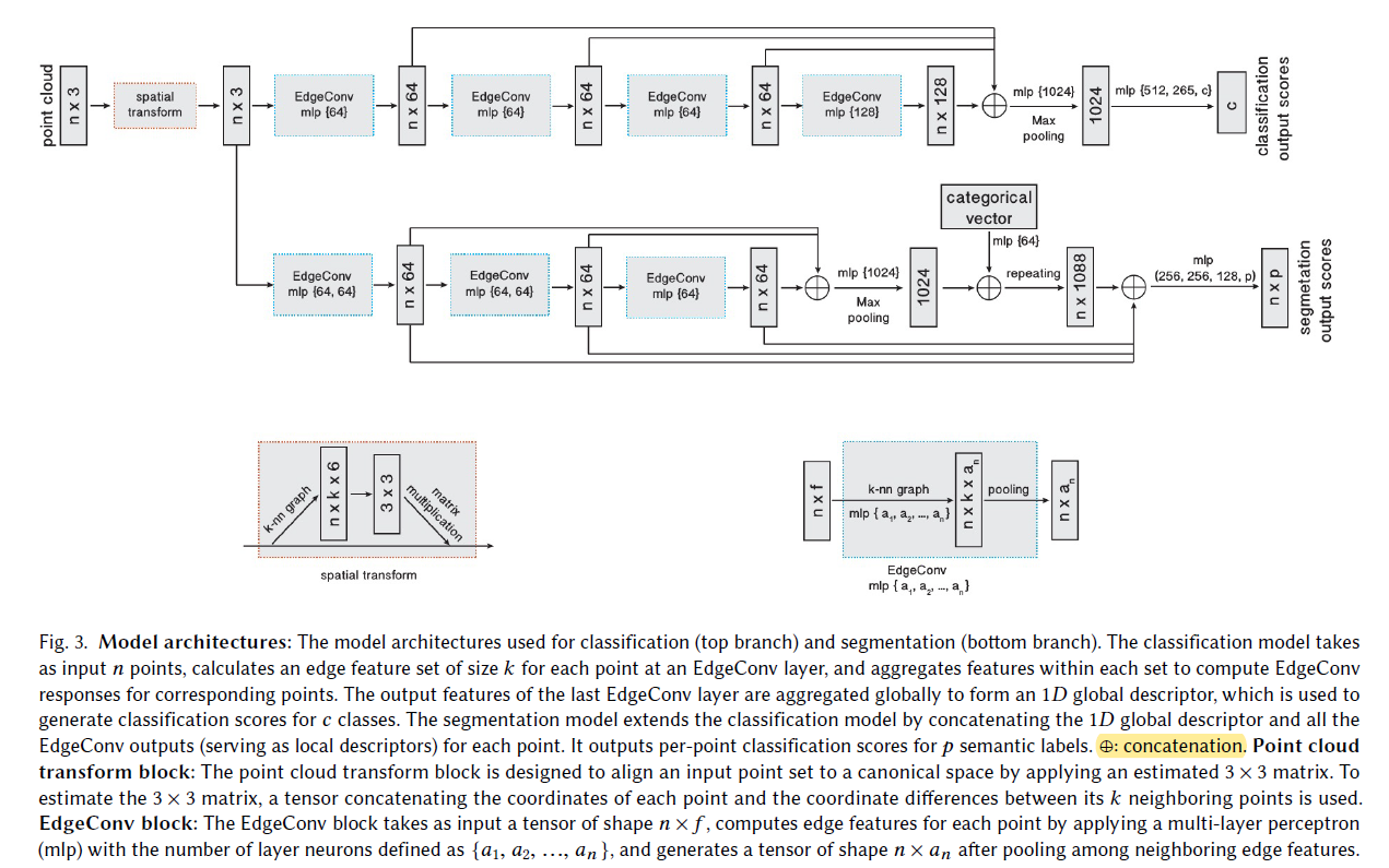
　　其整体的网络结构如下所示，值得注意的有：

• 整体的网络结构与PointNet的结构类似，最重要的区别就是使用EdgeConv代替MLP；
• 对于每个EdgeConv模块，我们即考虑全局特征，又考虑局部特征，（图2左）聚合函数 （图2右）；
  
• EdgeConv模块中KNN图的K值是一个超参，分类网络中K=20，而在分割网络中K=30；在做表格识别任务时，k=10；
• 在分割网络中，将global descripter和每层的local descripter进行连接后对每个点输出一个预测分数；
• 每层后的mlp全连接 都是为了计算边特征(edge features)，实现动态的图卷积。

  

## Edge Convolution

• 假设一个F维点$\mathbf{X}=\left\{\mathbf{x}_{1}, \ldots, \mathbf{x}_{n}\right\} \subseteq \mathbb{R}^{F}$， 最简单的$\mathrm{F}=3$(即x y z位置信息)，另外还可能引入每个点颜色、法线等信息。
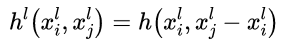
• 给定一个有向图 $\mathcal{G}=(\mathcal{V}, \mathcal{E})$ ，用来表示点云结构信息，其中顶点为$\mathcal{V}=\{1, \ldots, n\}$，边为 $\mathcal{E} \subseteq \mathcal{V} \times \mathcal{V}$，边特征函数$e_{i j}=h_{\Theta}\left(x_{i}, x_{j}\right)$，其中 $h$是 $\mathbb{R}^{F} \times \mathbb{R}^{F} \rightarrow \mathbb{R}^{F^{\prime}}$的映射(从结点信息获取边特征信息)
• 图2左 就描述了一个点$x_{i}$和其邻近点$x_{j}$ 的边特征$e_{i j}$求解过程，$h$使用三层全连接，用tf.layers.dense实现。(注：Dense and fully connected are two names for the same thing.)
• 图2右 描述的是结点参数更新的过程(结点聚合函数)，定义为$\square$，其定义是：$\mathbf{x}_{i}^{\prime}=\square_{j:(i, j) \in \mathcal{E}} h_{\Theta}\left(\mathbf{x}_{i}, \mathbf{x}_{j}\right)$，根据不同的需求，h和□有四种不同的选择
  • 认为$x_{i}$的特征是周围所有点的加权求和，这一点类似于图像的卷积操作，其中每个卷积核为${\theta}_{m}$，他的维度与x的维度相同，$\Theta=\left(\theta_{1}, \ldots, \theta_{M}\right)$表示所有卷积核的集合。其公式如下：$x_{i m}^{\prime}=\sum_{i=(j, j) \in \mathcal{E}} \boldsymbol{\theta}_{m} \cdot \mathbf{x}_{j}$
  • 若只考虑全局特征，即PointNet的使用方法，公式如下：$h_{\Theta}\left(\mathbf{x}_{i}, \mathbf{x}_{j}\right)=h_{\Theta}\left(\mathbf{x}_{i}\right)$
  • 若只考虑局部特征，即输入的仅为点和周围点的差，则公式如下：$h_{\Theta}\left(\mathbf{x}_{i}, \mathbf{x}_{j}\right)=h_{\Theta}\left(\mathbf{x}_{j}-\mathbf{x}_{i}\right)$
  • 同时关注全局特征和局部特征，这也是本文中的主要形式：$h_{\Theta}\left(\mathbf{x}_{i}, \mathbf{x}_{j}\right)=\bar{h}_{\Theta}\left(\mathbf{x}_{i}, \mathbf{x}_{j}-\mathbf{x}_{i}\right)$
    • 在本文中，h函数使用$e_{i j m}^{\prime}=\operatorname{ReLU}\left(\boldsymbol{\theta}_{m} \cdot\left(\mathbf{x}_{j}-\mathbf{x}_{i}\right)+\boldsymbol{\phi}_{m} \cdot \mathbf{x}_{i}\right)$，关系聚合函数选用 max

 

## 在表格识别任务中实现的代码  

 

 

 　　在我的毕设，即表格识别任务中，主要借用edge conv的思想，和分割部分的网络结构。

　　 其流程目的是将结点的特征进行提取，即输入为(25,900,133)（batch_size, node_num, feature_num），输出为经DGCNN处理后的结点信息,size为(25,900,128)，整体流程如下：

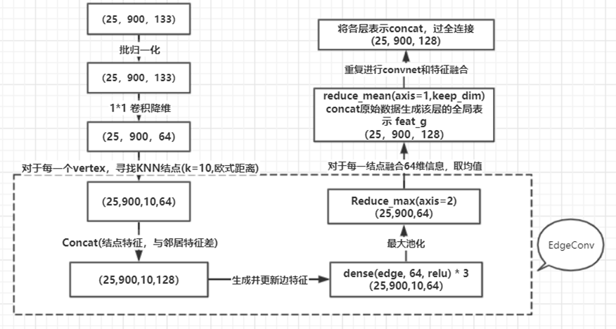
def edge_conv_layer(vertices_in, num_neighbors=30,
                          mpl_layers=[64, 64, 64],
                          aggregation_function=tf.reduce_max,
                          share_keyword=None,  # TBI,
                          edge_activation=None
                          ):
    trans_space = vertices_in  # (25,900,64)
    indexing, _ = indexing_tensor(trans_space, num_neighbors)  # (25,900,10,2)
    # change indexing to be not self-referential
    neighbour_space = tf.gather_nd(vertices_in, indexing)  # (25, 900, 10, 64)

    expanded_trans_space = tf.expand_dims(trans_space, axis=2)
    expanded_trans_space = tf.tile(expanded_trans_space, [1, 1, num_neighbors, 1])  # (25, 900 , 10（null）, 64)

    diff = expanded_trans_space - neighbour_space # (25, 900, 10, 64)
    edge = tf.concat([expanded_trans_space, diff], axis=-1)  # (25, 900, 10, 128)

    for f in mpl_layers:
        edge = tf.layers.dense(edge, f, activation=tf.nn.relu)  # 三层全连接 (25,900,10,64)
    if edge_activation is not None:
        edge = edge_activation(edge)

    vertex_out = aggregation_function(edge, axis=2)  # (25,900,64)
    # print("vertex_out:", vertex_out.shape)
    return vertex_out