DD出行供需分析和单量预测 2.0

背景描述
在出行问题上,中国市场人数多、人口密度大,总体的出行频率远高于其他国家,滴滴出行占领了国内绝大部分的网络呼叫出行市场,面对着巨大的数据量以及与日俱增的数据处理需求。为实现高频出行下的运力均衡,供需预测就是其中的一个关键问题。供需预测的目标是准确预测出给定地理区域在未来某个时间段的出行需求量及需求满足量。如果能预测到在未来的一段时间内某些地区的出行需求量比较大,就可以提前对营运车辆提供一些引导,指向性地提高部分地区的运力,从而提升乘客的整体出行体验。
一、问题需求
1. 不同地区24小时各时段供需是否匹配?(呼叫和应答情况、高频订单流向)
2. 高需求地区未来7天单量预测
二、数据来源与说明
数据来源:https://www.heywhale.com/mw/dataset/5f16971a94d484002d2a2eba/content
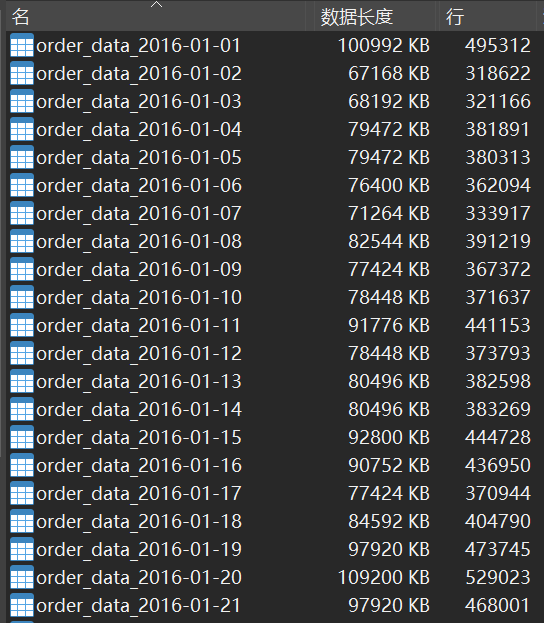
数据说明:训练数据集为M市2016年1月连续三周的打车出行数据信息(数据级850W+)。
具体数据如下,选取订单信息表、区域定义表、天气信息表进行分析。订单信息表
| 字段 | 类型 | 含义 | 示例 |
|---|---|---|---|
| order_id | string | 订单ID | 70fc7c2bd2caf386bb50f8fd5dfef0cf |
| driver_id | string | 司机ID | 56018323b921dd2c5444f98fb45509de |
| passenger_id | string | 用户ID | 238de35f44bbe8a67bdea86a5b0f4719 |
| start_district_hash | string | 出发地区域哈希值 | d4ec2125aff74eded207d2d915ef682f |
| dest_district_hash | string | 目的地区域哈希值 | 929ec6c160e6f52c20a4217c7978f681 |
| Price | double | 价格 | 37.5 |
| Time | string | 订单时间戳 | 2016-01-15 00:35:11 |
订单信息表主要覆盖了一张订单的基本信息,包括这张订单的乘客,以及接单的司机(driverid =NULL表示driverid为空,即这个订单没有司机应答),及出发地,目的地,价格和时间。
区域定义表
| 字段 | 类型 | 含义 | 示例 |
|---|---|---|---|
| district_hash | string | 区域哈希值 | 90c5a34f06ac86aee0fd70e2adce7d8a |
| district_id | string | 区域映射ID | 1 |
区域定义表主要表示区域的信息,结果需将区域哈希值映射为其相应的ID。
天气信息表
| 字段 | 类型 | 含义 | 示例 |
|---|---|---|---|
| Time | string | 时间戳 | 2016-01-15 00:35:11 |
| Weather | int | 天气 | 7 |
| temperature | double | 温度 | -9 |
| PM2.5 | double | pm25 | 66 |
天气信息表主要表示整个城市的每天间隔5分钟段的天气情况(实际采集数据有缺失,实际间隔时间有19min、7h不等,不能以统一5min间隔作为表连接条件)。其中的weather字段表示天气的实时描述信息,而温度以摄氏温度表示,PM2.5为实时空气污染指数。
指标定义
应答率:呼叫订单被应答的比例,应答订单/呼叫订单。
应答完单率:应答订单被完成订单比例,应答订单/完成订单。
三、导入数据
1.用Navicat将数据导入MySQL数据库。
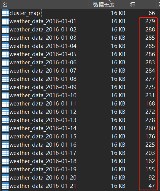
发现 weather表不同日期行数不一致,即每天的时间戳不等,先不合并,视需要情况而定。
2.查看表结构
desc `order_data_2016-01-01`;
desc `weather_data_2016-01-01`;
desc  cluster_map;
3.合并表信息(订单表、区域表)
3.1合并订单表、区域表
#新建空订单表
drop table if exists `order_data_2016_01`;
create  table `order_data_2016_01`(
order_id varchar(32)
,driver_id varchar(32)
,passenger_id varchar(32)
,start_district_hash varchar(32)
,dest_district_hash varchar(32)
,price double
,time datetime
);

#合并订单表
insert into order_data_2016_01
select * from `order_data_2016-01-01`
union all
select * from `order_data_2016-01-02`
union all
select * from `order_data_2016-01-03`
union all
select * from `order_data_2016-01-04`
union all
select * from `order_data_2016-01-05`
union all
select * from `order_data_2016-01-06`
union all
select * from `order_data_2016-01-07`
union all
select * from `order_data_2016-01-08`
union all
select * from `order_data_2016-01-09`
union all
select * from `order_data_2016-01-10`
union all
select * from `order_data_2016-01-11`
union all
select * from `order_data_2016-01-12`
union all
select * from `order_data_2016-01-13`
union all
select * from `order_data_2016-01-14`
union all
select * from `order_data_2016-01-15`
union all
select * from `order_data_2016-01-16`
union all
select * from `order_data_2016-01-17`
union all
select * from `order_data_2016-01-18`
union all
select * from `order_data_2016-01-19`
union all
select * from `order_data_2016-01-20`
union all
select * from `order_data_2016-01-21`
3.2 关联地址
#关联地址表,地址去哈希化(转为区域映射ID)
drop table if exists order_data_01;
select @i:=0;
create table order_data_01 as(
select
  (@i:= @i+1) as r1_id
  ,order_id
  ,driver_id
  ,passenger_id
  ,c1.district_id as start_id
  ,c2.district_id as dest_id
  ,price
  ,time
from order_data_2016_01
left join cluster_map c1
  on start_district_hash = c1.district_hash
left join cluster_map c2
  on dest_district_hash =c2.district_hash
);
四、数据清洗
4.1 检查重复值
drop table if exists order_data_02;
select @a:=0;
create table order_data_02 as(
with t1 as(
select
  *
  ,row_number()over(partition by order_id order by r1_id) as row_n
  ,count(order_id) over(partition by order_id order by r1_id) as cnt_n
from order_data_01
where r1_id > 0
)

#1 查看重复值
-- select
-- *
-- from t1
-- where r1_id > 0 and cnt_n>1
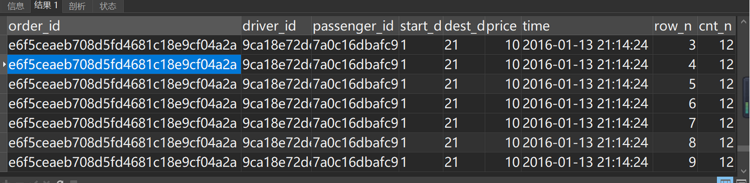
#2 去重复
select
  (@a:= @a+1) as r2_id
  ,order_id
  ,driver_id
  ,passenger_id
  ,start_id
  ,dest_id
  ,price
  ,time
from t1
where r1_id >0
  and row_n=1
);
4.2 检查空值
select
  sum(ISNULL(r2_id)) as r2_idn
  ,sum(ISNULL(order_id)) as order_idn
  ,sum(ISNULL(driver_id)) as driver_idn
  ,sum(ISNULL(passenger_id)) as passenger_idn
  ,sum(ISNULL(start_id)) as start_idn
  ,sum(ISNULL(dest_id)) as dest_idn
  ,sum(ISNULL(price)) as pricen
  ,sum(ISNULL(time)) as timen
from order_data_02
where r2_id >0 ;

目的地 dest_id 缺失 1346269 条数据,其他0缺失,目的地缺失id可能为未应答或已取消订单,暂不处理,实际业务可根据订单状态进一步判断。
4.3 检查异常值
# 查看数据整体情况,以及订单价格区间,时间范围,是否有异常
select
  count(1) as'订单数'
  ,count(distinct driver_id) as'司机数'
  ,count(distinct passenger_id) as'乘客数'
  ,min(price)
  ,max(price)
  ,min(time)
  ,max(time)
from order_data_02
where r2_id>0 and price < 1000000000 and time < '2029-02-01 00:00:00';

4.3.1 价格侧
#1 查看price=0 订单
select count(1) as '0元单量'
  ,concat(round((count(1)/8518049)*100,2),'%') as '0元单量占比'
from order_data_02
where  r2_id> 0
  and price= 0
  and time < '2029-02-01 00:00:00' ;

0元订单占比0.06%,可能是0元打车活动。

#查看最大价格price=1731 订单
select *
from order_data_02
where  r2_id>0
  and price= 1731
  and time < '2029-02-01 00:00:00';
 订单司机为空,属未应答订单。
#查看已接订单的价格TOP
select * from order_data_02
where  r2_id>0
  and price<1000000000
  and time < '2029-02-01 00:00:00'
  and  driver_id<>'NULL'
order by price desc limit 10 ;
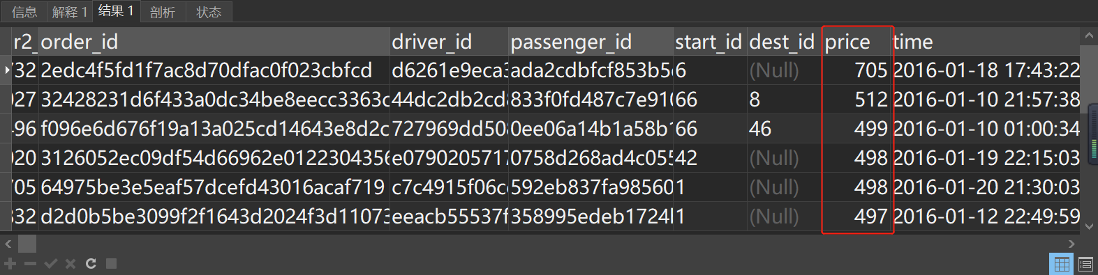
#查看705乘客的订单
select *
from order_data_02
where  r2_id>0
  and price<1000000000
  and time < '2029-02-01 00:00:00'
  and  driver_id <> 'NULL'
-- order by price desc limit 10
  and passenger_id= 'ada2cdbfcf853b5d4ae96c963631c50c' limit 50;
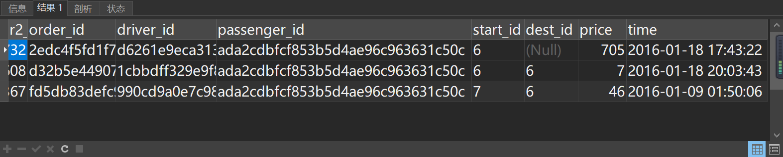
推测可能是专车,长途来回车程,加来回高速费。
4.3.2 乘客侧
#1 检查乘客侧打车次数
select
    passenger_id
    ,count(1) as'打车次数'
    ,count(1)/count(distinct date(time)) as '日均打车次数'
from order_data_02
where r2_id>0
    and time < '2029-02-01 00:00:00'
    and driver_id <>'NULL'
group by passenger_id
order by count(1) desc limit 10;
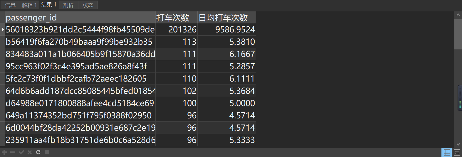
异常乘客 passenger_id='56018323b921dd2c5444f98fb45509de'  打车次数 201175,日均9587次。(官方反馈是因为之前通过其他方式叫车的部分用户没有登录,所以都是统一的ID,并不是数据问题)

#2 查看异常乘客订单明细
select *
from order_data_02
where r2_id>0
    and time < '2029-02-01 00:00:00'
    and driver_id <>'NULL'
    and passenger_id= '56018323b921dd2c5444f98fb45509de'
order by time
limit 20;
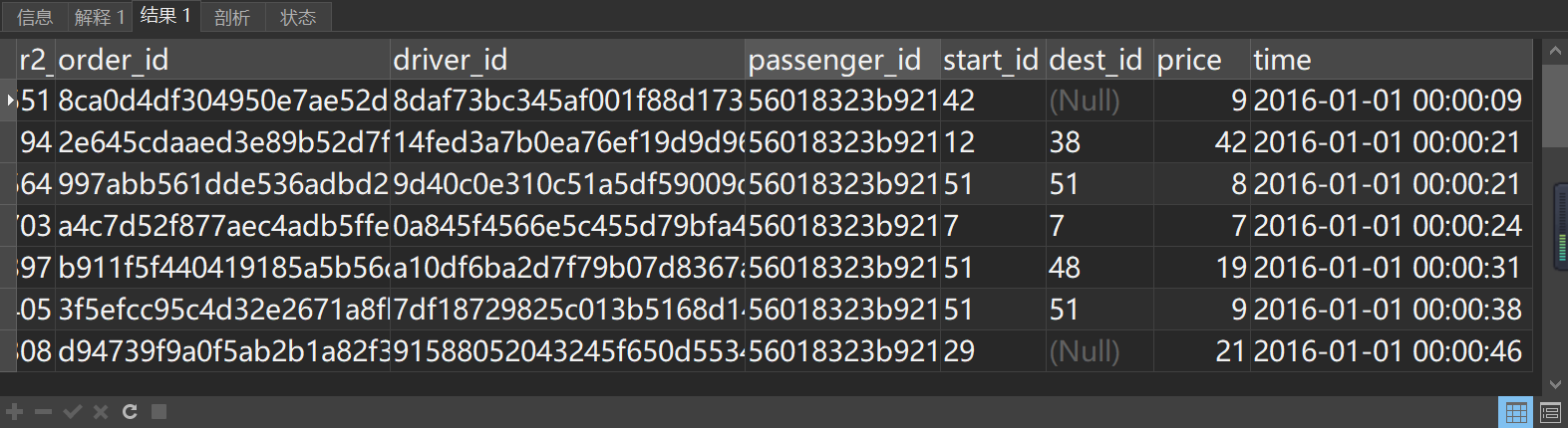
对该ID下的订单进一步核查发现同一时段内订单、司机、出发地均不一致,可以判定非同一乘客订单,先保留该数据,后续新增一列ID状态,将该ID产生的订单统一标记为:异常乘客ID。
4.3.3 司机侧
#1 司机侧检查接单次数
select
    driver_id
    ,count(1) as '接单次数'
    ,count(1)/count(distinct date(time)) as '日均接单次数'
from order_data_02
where r2_id>0
    and driver_id <> 'NULL'
    and time < '2029-02-01'
group by driver_id
order by '日均接单次数' desc limit 50;
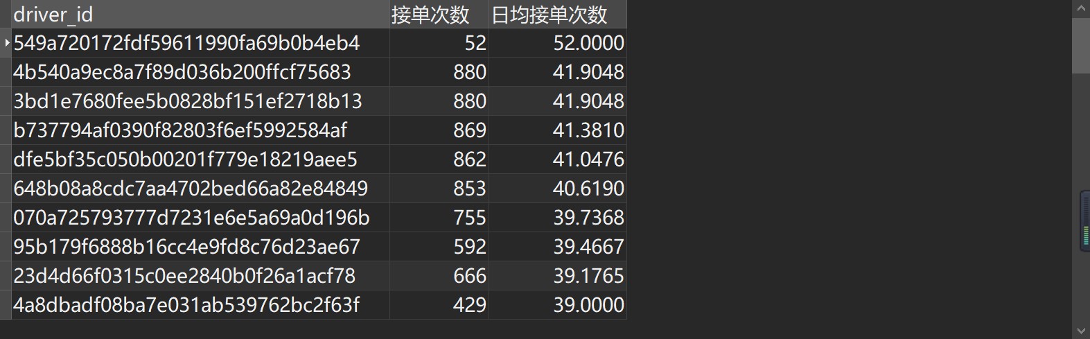
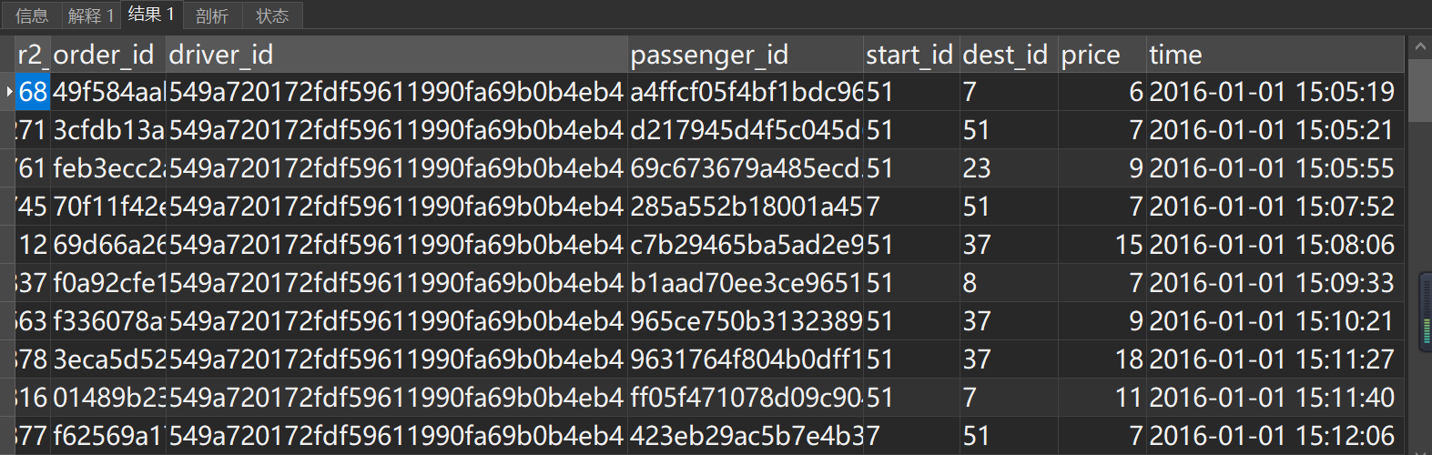
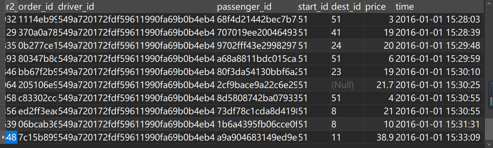
 #异常司机driver_id ='549a720172fdf59611990fa69b0b4eb4' 接单明细
select
  *
from order_data_02
where r2_id > 0
    and driver_id ='549a720172fdf59611990fa69b0b4eb4'
    and time < '2029-02-01'
order by time limit 100;
#对异常司机driver_id ='549a720172fdf59611990fa69b0b4eb4'进一步核查
select
  count(distinct start_id) as start_id_n
  ,count(distinct dest_id) as dest_id_n
  ,count(distinct order_id) as order_id_n
  ,min(time)
  ,max(time)
from order_data_02
where r2_id >0
    and driver_id ='549a720172fdf59611990fa69b0b4eb4'
    and time <'2026-02-01 00:00:00'
order by time;

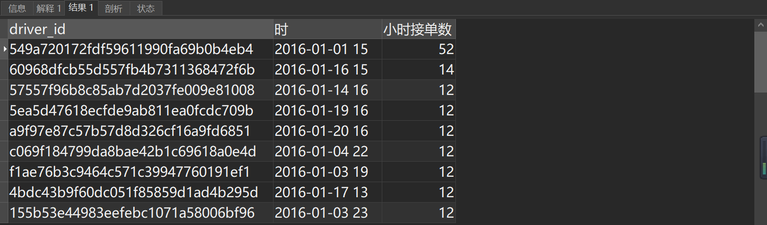
司机 driver_id ='549a720172fdf59611990fa69b0b4eb4' 在1月1日15:05-15:33期间合计接单数52,接单地2个,目的地12个,平均每分钟1.9单,接单频率异常,可能为测试单,稍后剔除处理。

#筛查1小时内接单10次以上的司机
select driver_id
  ,date_format(time,'%Y-%m-%d %H') as '时'
  ,count(order_id) as '小时接单数'
  from order_data_02
where r2_id >0
    and driver_id <>'NULL'
    and time <'2026-02-01'
group by 1,2 having count(order_id) >10
order by 3 desc
  limit 100;
共21条记录,因无法判断业务类型(专车/拼车/顺风车)及订单状态(取消/完成),对其他订单均保留处理。
#2 异常值处理:标记状态(订单状态order_status,乘客id状态pid_status),删除异常司机id数据。
#标记状态,order_status和pid_status
-- driver_id='NULL' 为未应答;
-- passenger_id= '56018323b921dd2c5444f98fb45509de' 为乘客id异常
drop table if exists order_data;
create table order_data as(
select
  *
  ,case when driver_id='NULL' then '未应答' else '已接单' end as order_status
  ,case when passenger_id= '56018323b921dd2c5444f98fb45509de' then '乘客id异常' else '正常' end as pid_status
from order_data_02
where r2_id >0
    and time<'2026-02-01 00:00:00'
);

#删除driver_id ='549a720172fdf59611990fa69b0b4eb4'数据
delete from order_data
where driver_id ='549a720172fdf59611990fa69b0b4eb4'
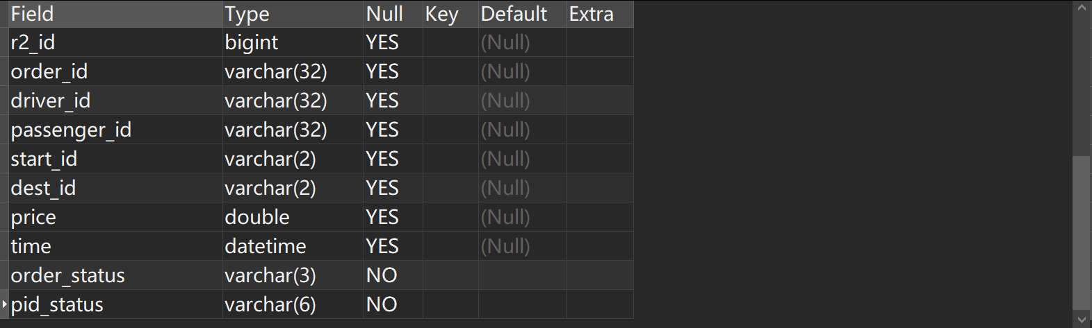
#查看清洗后的数据结构
desc order_data;
五、解决问题
5.1 运营情况
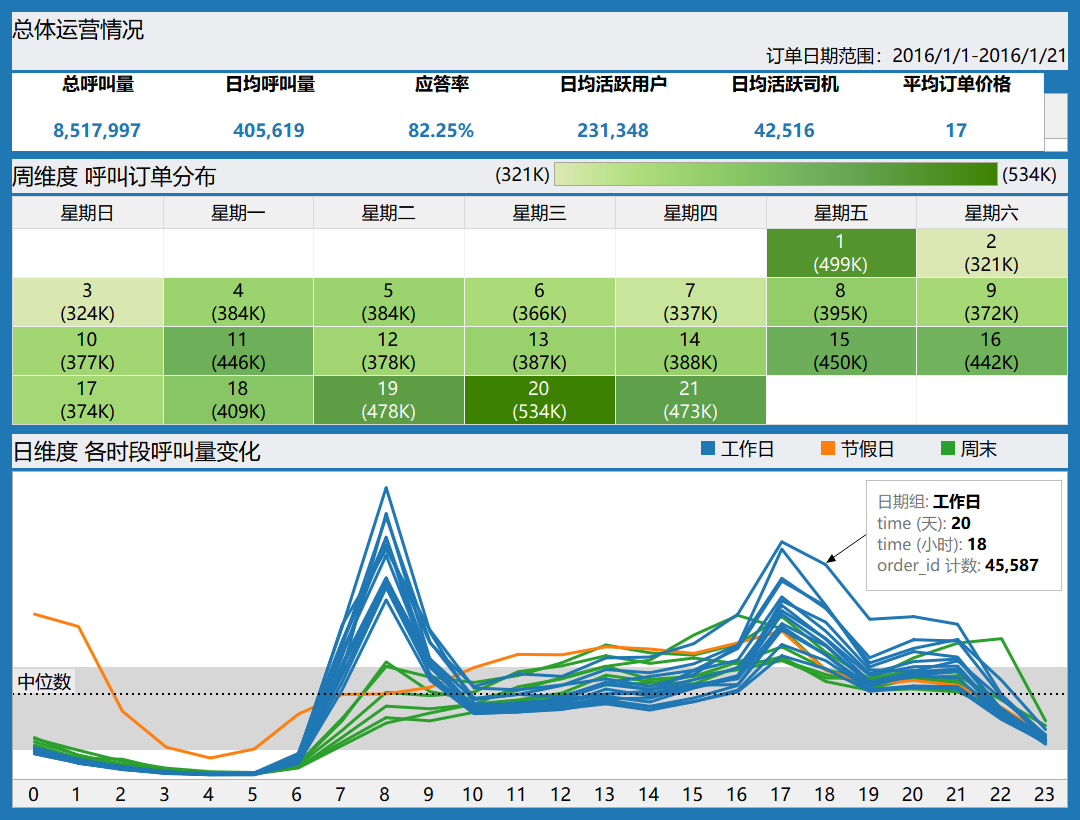
总体运营情况 (2016年1月1日-1月21日)
在此期间,M市运营数据如下:
-
呼叫量:累计约851.8万单,日均约40.6万单。
-
应答情况:整体应答率为82.25%。
-
用户与司机活跃度:日均活跃用户达23.1万,日均活跃司机4.3万。
-
订单价格:平均每单价格为17元。
周维度分析
-
周期性:三周数据显示,周一至周日的总呼叫量未呈现明显的周期性规律。
-
波动高点:1月1日(元旦)以及1月19日,20日,21日的呼叫量相对较高。
-
波动低点:工作日中,1月7日的呼叫量为三周最低。
日维度分析
- 常态趋势:非节假日期间,每日23时至次日6时为订单低谷。7时起呼叫量开始爬升,早高峰集中于8时,晚高峰则主要在17时。早晚高峰的呼叫量在工作日显著高于周末。
- 周末特征:周末全天的订单增长曲线相对工作日更为平缓。
- 节假日异常:元旦当天(1月1日)的0时至6时,呼叫量显著高于非节假日同时段,呈现异常峰值。
- 日间对比:在10时至14时日间时段,不同日期类型的呼叫量波动趋势呈现出 节假日 > 周末 > 工作日 的特征,这可能与休息日出行需求的增加有关。
5.2 高峰期供需匹配分析
5.2.1 工作日与非工作日呼叫、应答情况?
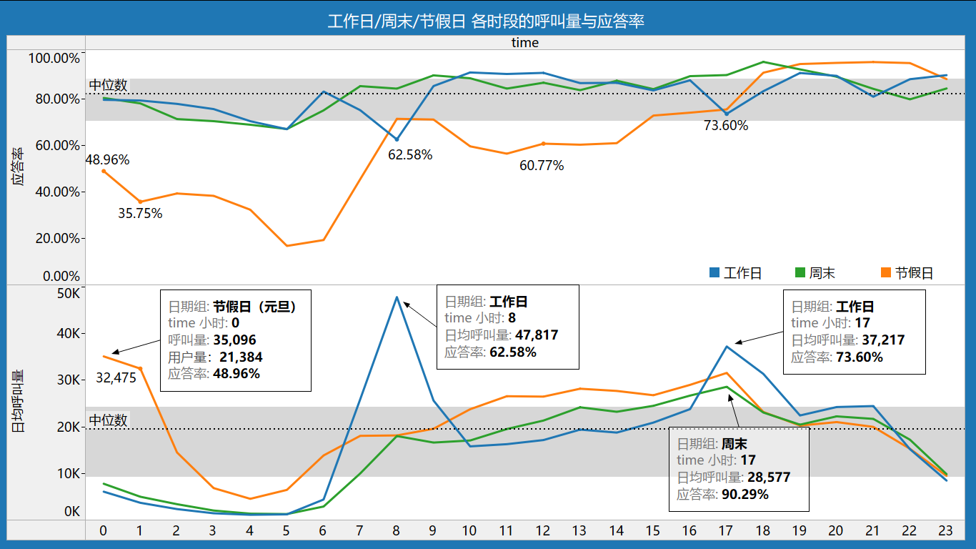
从呼叫、应答率看,供需关系在不同时段呈现显著差异:
- 工作日早晚高峰供需紧张
早高峰(8时)日均呼叫量达4.8万,应答率仅为62.58%;晚高峰(17时)日均呼叫量3.7万,应答率为73.60%,均反映出明显的供不应求状况。
- 周末白天供需相对平衡稳定
在7时至19时时段内,应答率持续高于80%,该时段供需匹配良好,运行平稳。
- 节假日(元旦)供给严重不足
1)凌晨时段:0时与1时的呼叫量分别达3.5万和3.2万,约为周末同期的4倍,而应答率骤降至48.96%和35.75%,供给缺口极大;
2)日间时段:11时至17时呼叫量较周末小幅上升,但应答率仍仅维持在60%-70%的偏低区间,供给能力持续不足。
供需失衡的可能原因:
-
供给短缺:热点区域司机资源在高峰期无法满足集中爆发的需求。
-
需求过载:乘客需求在特定时段和区域过于密集,导致运力瞬时承压。
-
环境制约:恶劣天气、道路拥堵或交通管制等客观因素,降低了司机响应与到达效率。
-
意愿与效能:司机接单积极性不足,或服务效率有待提升,影响整体应答水平。
优化策略:
- 动态激励与调价
1)在高峰热点区域实施更具吸引力的激励政策(如佣金补贴、专项奖励),提升司机接单意愿。
2)基于实时供需数据动态调整订单价格,以价格信号引导运力调配,提升应答积极性。
- 需求引导与分流
鼓励拼车出行,通过优惠券、积分等激励措施,分散即时性独乘需求。
-
派单机制优化
根据实时呼叫需求,动态调整派单范围及订单匹配优先级,缩短乘客等待时间,提升整体服务效率。
-
运力预测与调度
1)运用数据模型预测高峰期需求分布,提前向热点区域调配运力。
2)加强热点区域的司机招募与定向运营,持续扩充及优化该区域司机供给。
5.2.3 地区各时段供需分析
要进行聚类分析的输入
| 群集 | 项数 | 中心呼叫量 | ||||||
| 低呼叫量地区 | 53 | 1834 | ||||||
| 中等呼叫量地区 | 10 | 17323 | ||||||
| 高呼叫量地区 | 3 | 45046 | ||||||
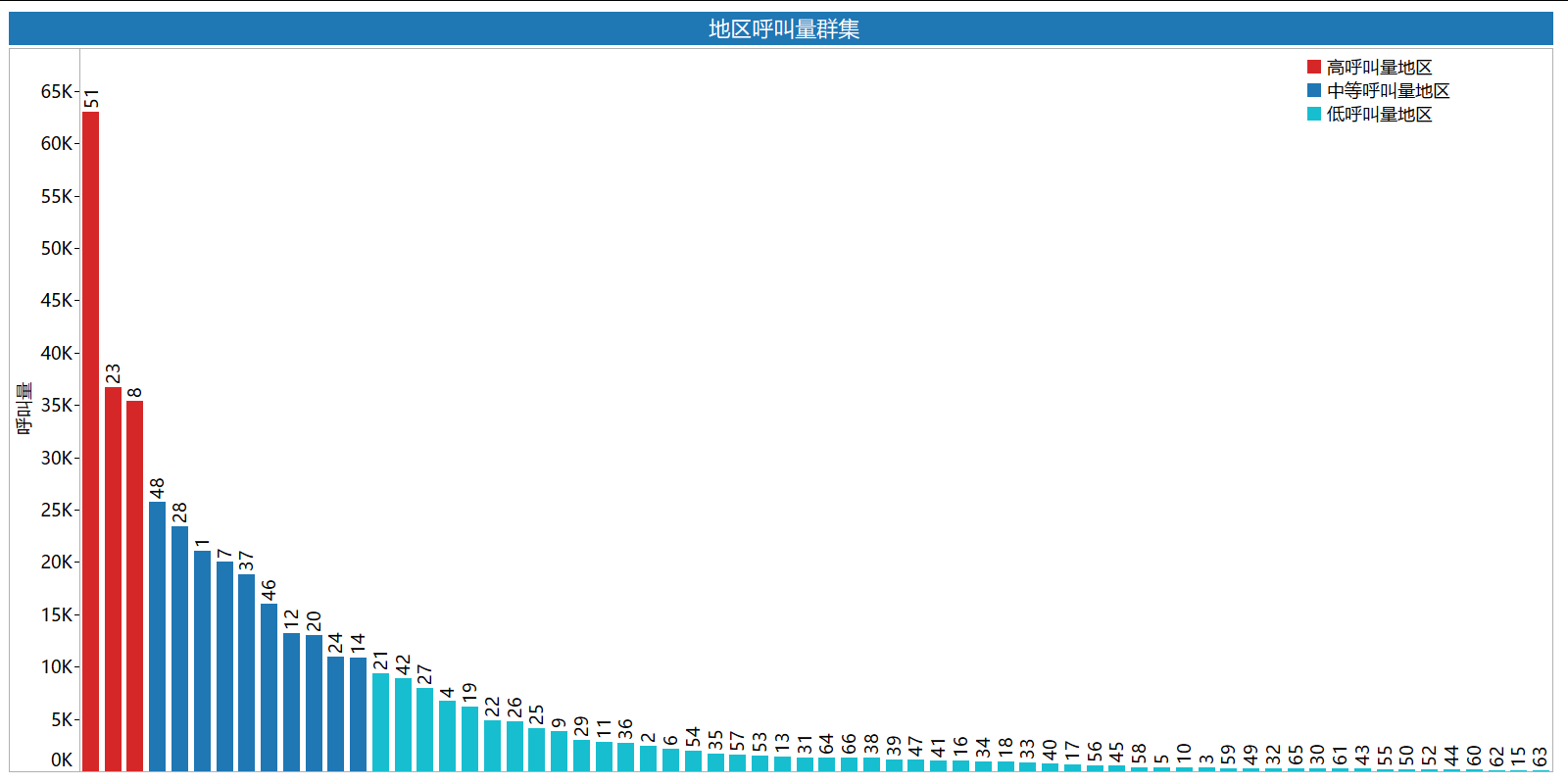
依据呼叫量对地区进行分群:
- 高呼叫量地区id:51 > 23 > 8;
- 中等呼叫量地区id:48 > 28 > 1 > 7 > 37 > 46 > 12 > 20 > 24 > 14;
- 低呼叫量地区id:21 > 42 > 27 > 4 >19 >22 > 26 > 25 > 9 >29 >11.....
5.2.3.1 工作日(高、中高呼叫量)地区各时段日均呼叫量和应答率
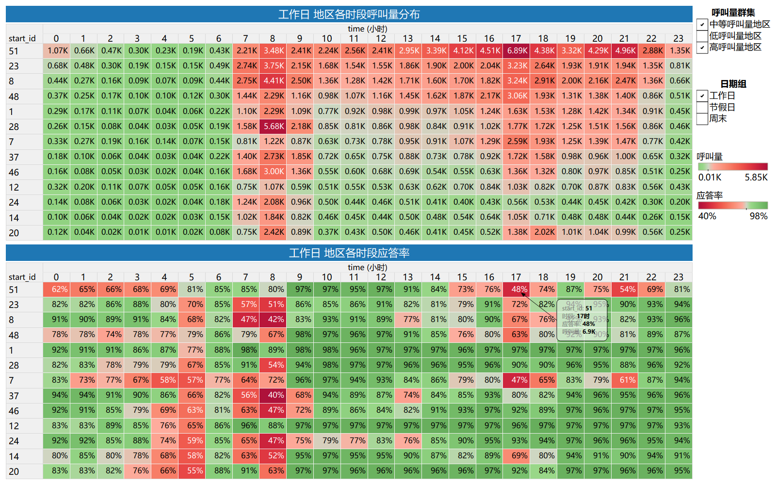 工作日供需紧张,需重点补充运力的地区及对应时段如下:
| 地区ID | 7时-23时 需重点补充运力时段 | 0时-6时 (凌晨低峰)需适当补充运力时段 |
|---|---|---|
| id51 | 0时, (15时-18时), (20时-22时) | 0时-1时(重点),2时-4时 |
| id23 | (7时-8时), 15时, (17时-18时) | 5时 |
| id8 | (7时-8时), 13时, (17时-18时) | 5时 |
| id48 | (7时-8时), 15时, 17时 | 0时-5时 |
| id1 | 无 | 5时 |
| id28 | 8时 | 2时-5时 |
| id7 | (7时-8时), 15时, (17时-18时), (20时-21时) | 1时-6时 |
| id37 | (7时-9时), 13时 | 5时 |
| id46 | (7时-9时) | 3时-5时 |
| id12 | 无 | 4时-5时 |
| id24 | (7时-11时), 13时 | 4时-5时 |
| id14 | (7时-8时), 17时 | 3时-5时 |
| id20 | 8时 | 3时-5时 |
工作日运力紧张时段主要集中在早晚高峰 (7时-9时) 与 (17时-18时)。其中部分区域(如 id51、id48、id7)高峰提前至 15时开始并延续至18时,且 id51 与 id7 在 夜间(20时-22时) 仍存在明显出行高峰。
5.2.3.2 周末(高、中高呼叫量)地区各时段日均呼叫量和应答率
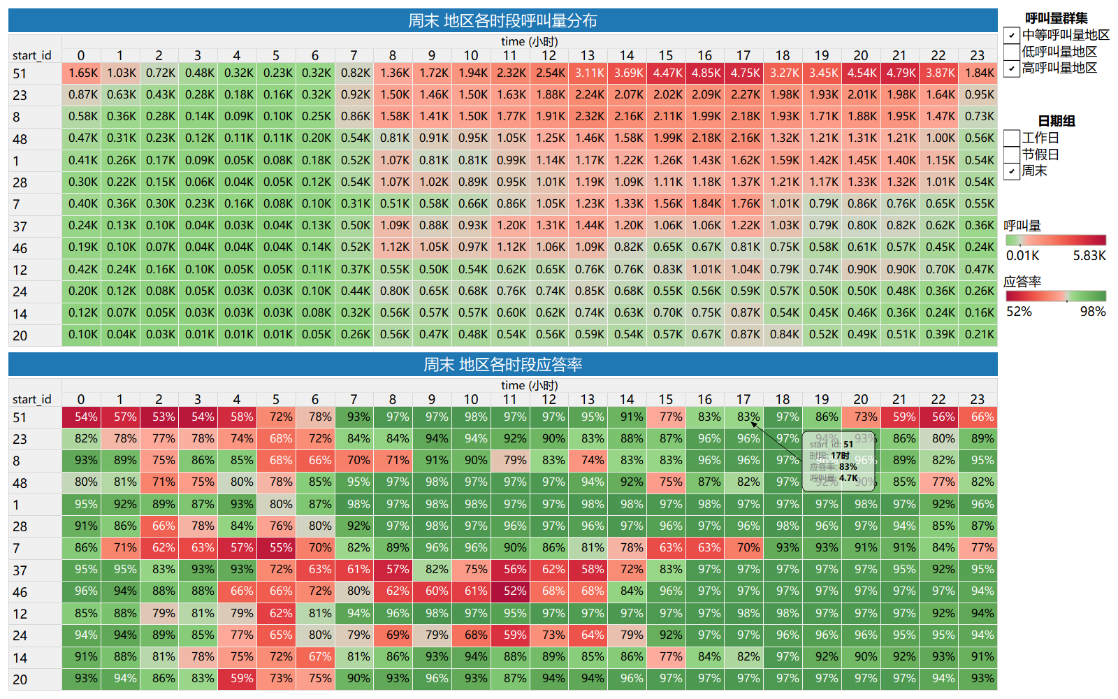
周末供需紧张,需重点补充运力的地区时段如下:
| 地区ID | 重点补充运力时段 |
|---|---|
| id51 | 0时-2时, 15时, 20时-23时 |
| id23 | 1时 |
| id8 | 7时-8时, 11时, 13时 |
| id48 | 15时, 22时 |
| id1 | 无 |
| id28 | 无 |
| id7 | 14时-17时, 23时 |
| id37 | 7时-8时, 10时-14时 |
| id46 | 8时-13时 |
| id12 | 无 |
| id24 | 7时-14时 |
| id14 | 15时 |
| id20 | 无 |
周末出行模式与工作日存在显著差异,地区id37,46,24在7时至14时持续长时间运力供给匮乏。地区id7在14时-17时出现午后小高峰,需运力支援。id51在20时-22时出现晚高峰,0时-4时应答率低于60%,夜间服务车辆不足。周末运力紧张的本质是 “休闲消费驱动的时空需求集聚”,运营重心应从工作日的“通勤保障”转向周末的“场景化供需匹配”。
5.2.3.3 节假日(高、中高呼叫量)地区各时段呼叫量和应答率
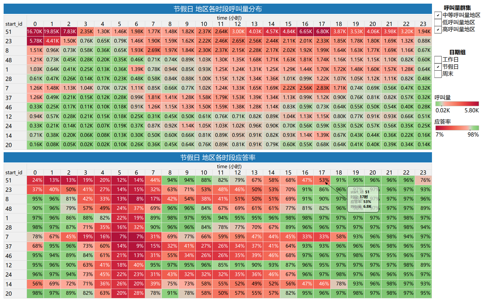
节假日(元旦)供需紧张,需重点补充运力的地区时段整理如下:
| 地区ID | 重点补充运力时段 |
|---|---|
| id51 | (0时-7时), (12时-17时), 23时 |
| id23 | (0时-15时) |
| id8 | (5时-15时) |
| id48 | 7时, (11时-15时) |
| id1 | 6时 |
| id28 | (11时-14时) |
| id7 | (0时-18时) |
| id37 | 0时, (6时-15时) |
| id46 | (6时-15时) |
| id12 | 无 |
| id24 | (7时-15时) |
| id14 | 0时,(7时-18时) |
| id20 | (9时-14时) |
节假日(元旦)期间出行需求集中,部分地区(如id7、id23、id37、id46等)供需紧张时段覆盖全天大部分时间,尤其集中在上午至傍晚(6时-18时),同时多个区域凌晨及深夜时段(如id51的0时-7时)也存在明显运力缺口。
5.2.3.4 定位不同日期类型(工作日、周末、节假日) 需要补充运力的时段和地区,查看其订单流向分布(出发地 star_id→ 目的地 dest_id) 特征,确定密集订单流线路,合理调配运力 如:
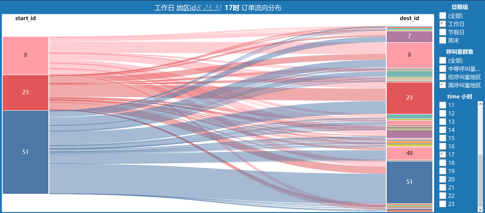
工作日高呼叫量地区17时,
1)以地区Id 51为核心的高频线路 (出发地 star_id→ 目的地 dest_id)
-
51 → 51(区域内部出行)
-
51 → 23
-
51 → 48
-
51 → 8
-
51 → 7
2)以地区Id 23为核心的高频线路
-
23 → 23(区域内部出行)
-
23 → 51
-
23 → 8
3) 以地区Id 8为核心的高频线路
-
8 → 8(区域内部出行)
-
8 → 23
-
8 → 51
-
8 → 37
-
8 → 7
可以发现,高呼叫量地区区域内部出行频次最高,而需求整体 跨区出行需求 > 区域内部出行需求,同时跨区出行存在双向高频线路,如 :
工作日17时,地区id 51订单流出线路分布:
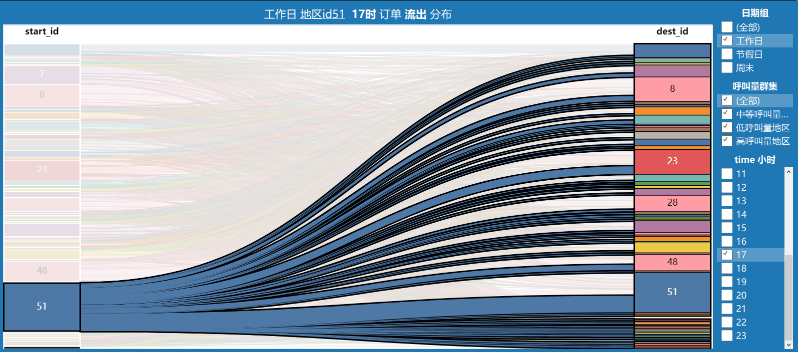
工作日17时,地区id 51订单流入线路分布:
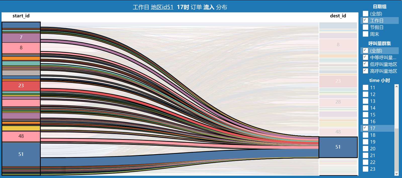
17时高频线路,如51 → 51(内部循环),51 ↔ 23(双向高频),51 ↔ 8(双向高频)。
id 51是强需求区,持续供不应求;id 23 和 id 8是次核心区;51 → 8 需求 > 8 →51需求,51 → 23 需求 > 23 →51需求,51车辆回流少,为保障51区运力蓄水,调度系统必须保证回流速度足够快,即 外区车辆返回时间短、回流比例高,所有区域回流51区的订单调度优先级需调至最高级。
5.2.3.5 运力分配策略
5.2.3.5.1 计算运力配比(基于历史数据)假设地区id51总运力车辆数为 N,历史订单比例约为:
D51→51 : D51→外区 : D外区 → 51 = 2 : 4.5 : 3.5
#AI 建模输出
一、稳态建模与平衡分析 已知订单比例(相对值) D5151= 2.0, D51out= 4.5, Din51 = 3.5 自然流出与流入: 流出 51 区的车辆数(因订单) D51out = 4.5 流入 51 区的车辆数(载客订单) Din51 = 3.5 自然净流出 = 4.5−3.5 = 1.0 所以必须额外 空驶调度 回流车辆数: S = 1.0 即该时段需从外区空驶调回 1.0 比例的车,才能使车辆分布稳定。 总任务比例(需要车辆时间的行程) D5151= 2.0 D51out = 4.5 Din51 = 3.5 空驶调度回流 S=1.0 Rtotal = 2.0 + 4.5 + 3.5 + 1.0 = 11.0
二、车辆分布比例 按任务执行的位置分类: 在 51 区内执行的任务(起点在 51): D5151 + D51out = 2.0 + 4.5 = 6.5 在外区执行的任务(起点在外区): Din51 + S = 3.5 + 1.0 = 4.5 总任务比例 = 11.0。 车辆在 51 区内的时间占比: 6.5/11.0 ≈ 59.1% 在外区的时间占比: 4.5/11.0 ≈ 40.9% 稳态下,车辆数的分布比例应与时间占比一致(假设各任务平均时长相同): N51:N外 = 6.5 : 4.5 = 13 : 9 (≈ 59.1%:40.9%) 即: N51 ≈ 0.591 N, N外 ≈ 0.409 N 三、供需匹配与所需总车辆 N 设实际每小时订单总量为 Q,已知比例: D5151 : D51out : Din51 = 2 : 4.5 : 3.5 所以: Q5151 = 0.2Q Q51out = 0.45Q Qin51 = 0.35Q 总载客任务数: Q载客 = Q5151 + Q51out + Qin51 = Q 总空驶任务数(单位时间): Q空驶 = S × Q/10 = 1.0× Q/10 =0.1Q 总任务数: Q总任务 = Q + 0.1Q = 1.1Q 平均每单时长t,车辆平均利用率为 U: N = 1.1Qt / U 举例: 设 Q = 1000Q = 1000 单/小时,t=0.2 小时,U=0.7: N = 1.1×1000×0.2 / 0.7 ≈314 辆车 N51 ≈ 0.591×314 ≈ 185 N外 ≈ 314−185 = 129
5.2.3.5.2 运力分配策略
策略目标:维持约 59% 的车辆在 51 区内,41% 在外区。
提升 外区 → 51 的载客订单比例,减少空驶成本。
1)实时监控指标
-
核心指标:51区车辆占比(目标 58%~60%)。
-
预警线:<58% 时触发调度,>60% 时允许更多流出。
-
回流载客比例:目前 3.5/4.5 ≈ 77.8%,可优化至 >80% 减少空驶。
2)调度规则
派单优先级
| 订单类型 | 优先级 | 派给谁 | 目标 |
|---|---|---|---|
| 51→51 | 高 | 51区内空闲车辆 | 快速服务,维持区内循环 |
| 51→外区 | 中 | 51区内车辆(若占比>58%) | 防止过度流出 |
| 外区→51 | 最高 | 外区空闲车辆 | 促进回流,减少空驶 |
调度触发机制
-
当 51 区占比 < 58%:
-
限制 51→外区 长单,启用 拼车模式优先,减少车辆流出。
- 加强回流调度,对外区(邻近区域) 闲置 > 5 分钟 的车辆发起 空驶回51 指令(司机端可设补贴激励)。
-
提高外区→51 订单的司机奖励。
-
-
当 51 区占比 > 60%:
1. 放宽 51→外区 的派单限制,允许更多车流出。
2. 降低空驶补贴。
3)车队分组建议
-
51 区核心车队(约 60% N):主要服务 51→51 短单,部分接 51→外区 长单(若占比允许)。
-
跨区车队(约 40% N):在外区服务返回订单,平衡流动。
4) 定价与激励
- 51→外区:价格可设基准或微涨,因需求旺盛。
-
外区→51:给予乘客优惠(例如 9 折),鼓励下单提高载客回流,减少空驶。
- 51→51:基准价。
5)持续调优:监控应答率、车辆利用率、回流比例,每周优化参数。
5.3 地区未来7天单量预测
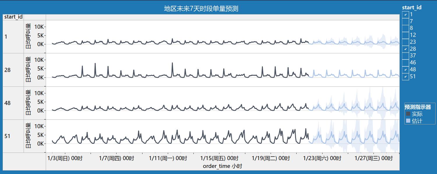
用于创建预测的选项
| 时间系列: | order_time 小时 |
| 度量: | 日均呼叫量 |
| 向前预测: | 169 小时 (2016年1月21日 下午11 – 2016年1月28日 下午11) |
| 预测依据: | 2016年1月9日 下午9 – 2016年1月21日 下午10 |
| 忽略最后: | 1 小时 (2016年1月21日 下午11) |
| 季节模式: | 24 小时周期 |
| 行 | 初始 | 从初始值更改 | 季节影响 | 贡献 | |||||||
| start_id | 2016年1月21日 下午11 | 2016年1月21日 下午11 – 2016年1月28日 下午11 | 高 | 低 | 趋势 | 季节 | 质量 | ||||
| 1 | 443 | ± | 140 | -6 | 2016年1月28日 上午8 | 2 | 2016年1月28日 上午4 | 0 | 95.8% | 4.2% | 好 |
| 28 | 601 | ± | 291 | -1 | 2016年1月28日 上午8 | 4 | 2016年1月28日 上午4 | 0 | 13.4% | 86.6% | 确定 |
| 48 | 581 | ± | 190 | 131 | 2016年1月28日 下午5 | 3 | 2016年1月28日 上午3 | 0 | 100.0% | 0.0% | 确定 |
| 51 | 1,182 | ± | 421 | 110 | 2016年1月28日 下午5 | 3 | 2016年1月28日 上午5 | 0 | 100.0% | 0.0% | 确定 |
通过对地区id为1、28、48、51进行的预测分析,发现tableau预测存在一定局性性,其季节模式(周期性)仅考虑24小时,未体现7天周期性,实际周末时段与工作日时段出行高峰期不同(周六和周日早高峰单量实际较工作日有所减少),故不具备参考价值。
解决思路:再剔除元旦数据的基础上,把工作日和周末单独提取出来,重命名日期使其连续,再分别预测。
5.3.1 高呼叫量地区工作日订单预测


drop table if EXISTS order_weekday;
create table order_weekday as(
select
order_id
,start_id
,time
from order_data
where date_format(time,'%w') in (1,2,3,4,5)
)

delete from order_weekday where DATE_FORMAT(time,'%Y-%m-%d') = '2016-01-01'
update order_weekday set time = replace(time,'2016-01-15','2016-01-17') where DATE_FORMAT(time,'%Y-%m-%d') < '2026-02-01';
update order_weekday set time = replace(time,'2016-01-14','2016-01-16') where DATE_FORMAT(time,'%Y-%m-%d') < '2026-02-01';
update order_weekday set time = replace(time,'2016-01-13','2016-01-15') where DATE_FORMAT(time,'%Y-%m-%d') < '2026-02-01';
update order_weekday set time = replace(time,'2016-01-12','2016-01-14') where DATE_FORMAT(time,'%Y-%m-%d') < '2026-02-01';
update order_weekday set time = replace(time,'2016-01-11','2016-01-13') where DATE_FORMAT(time,'%Y-%m-%d') < '2026-02-01';
update order_weekday set time = replace(time,'2016-01-08','2016-01-12') where DATE_FORMAT(time,'%Y-%m-%d') < '2026-02-01';
update order_weekday set time = replace(time,'2016-01-07','2016-01-11') where DATE_FORMAT(time,'%Y-%m-%d') < '2026-02-01';
update order_weekday set time = replace(time,'2016-01-06','2016-01-10') where DATE_FORMAT(time,'%Y-%m-%d') < '2026-02-01';
update order_weekday set time = replace(time,'2016-01-05','2016-01-09') where DATE_FORMAT(time,'%Y-%m-%d') < '2026-02-01';
update order_weekday set time = replace(time,'2016-01-04','2016-01-08') where DATE_FORMAT(time,'%Y-%m-%d') < '2026-02-01';
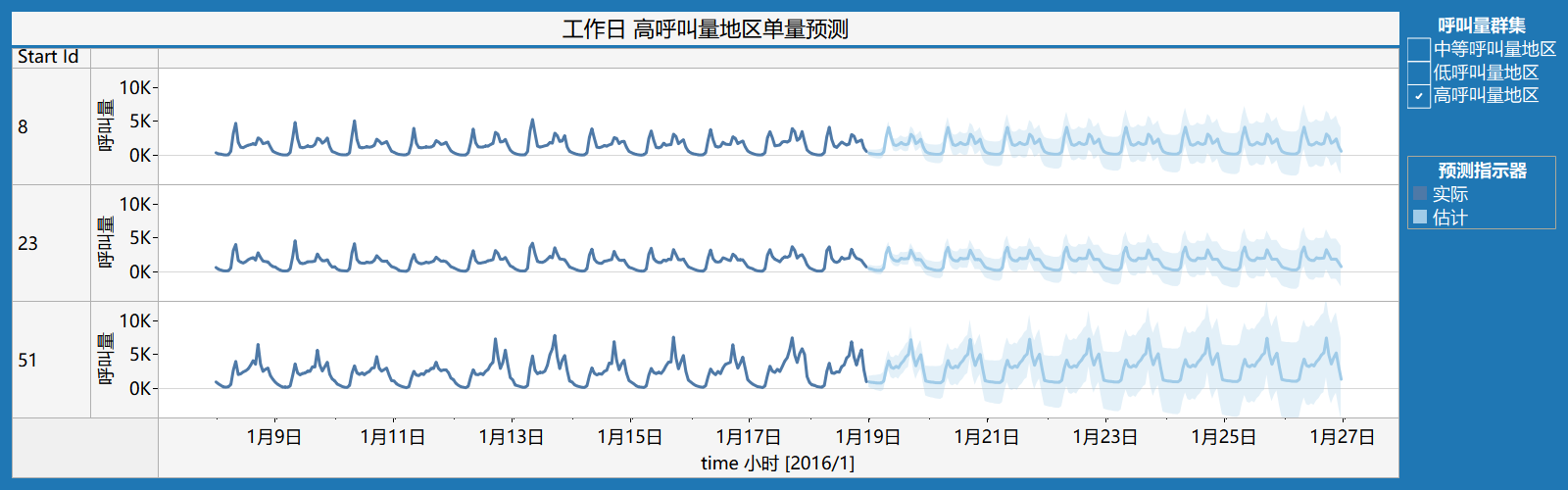
| 时间序列: | time 小时 |
| 度量: | 呼叫量 |
| 向前预测: | 192 小时 (2016年1月19日 0时 – 2016年1月26日 23时) |
| 预测依据: | 2016年1月8日 0时 – 2016年1月18日 23时 |
| 忽略最后: | 72 小时 (2016年1月19日 0时 – 2016年1月21日 23时) |
| 季节模式: | 24 小时周期 |
工作日(1/22,1/25-1/28)高呼叫量地区单量预测和质量评估:
| 行总和 | 初始 | 从初始值更改 | 季节影响 | 贡献 | |||||||
| Start Id | 2016年1月19日 0时 | 2016年1月19日 0时 – 2016年1月26日 23时 | 高 | 低 | 趋势 | 季节 | 质量 | ||||
| 8 | 354 | ± | 482 | 258 | 2016年1月26日 8时 | 2,597 | 2016年1月26日 4时 | -1,367 | 0.0% | 100.0% | 良好 |
| 23 | 536 | ± | 460 | 258 | 2016年1月26日 8时 | 2,066 | 2016年1月26日 4时 | -1,322 | 0.1% | 99.9% | 良好 |
| 51 | 1,005 | ± | 842 | 378 | 2016年1月26日 17时 | 4,202 | 2016年1月26日 5时 | -2,162 | 0.2% | 99.8% | 良好 |
5.3.2 中等呼叫量地区工作日订单预测
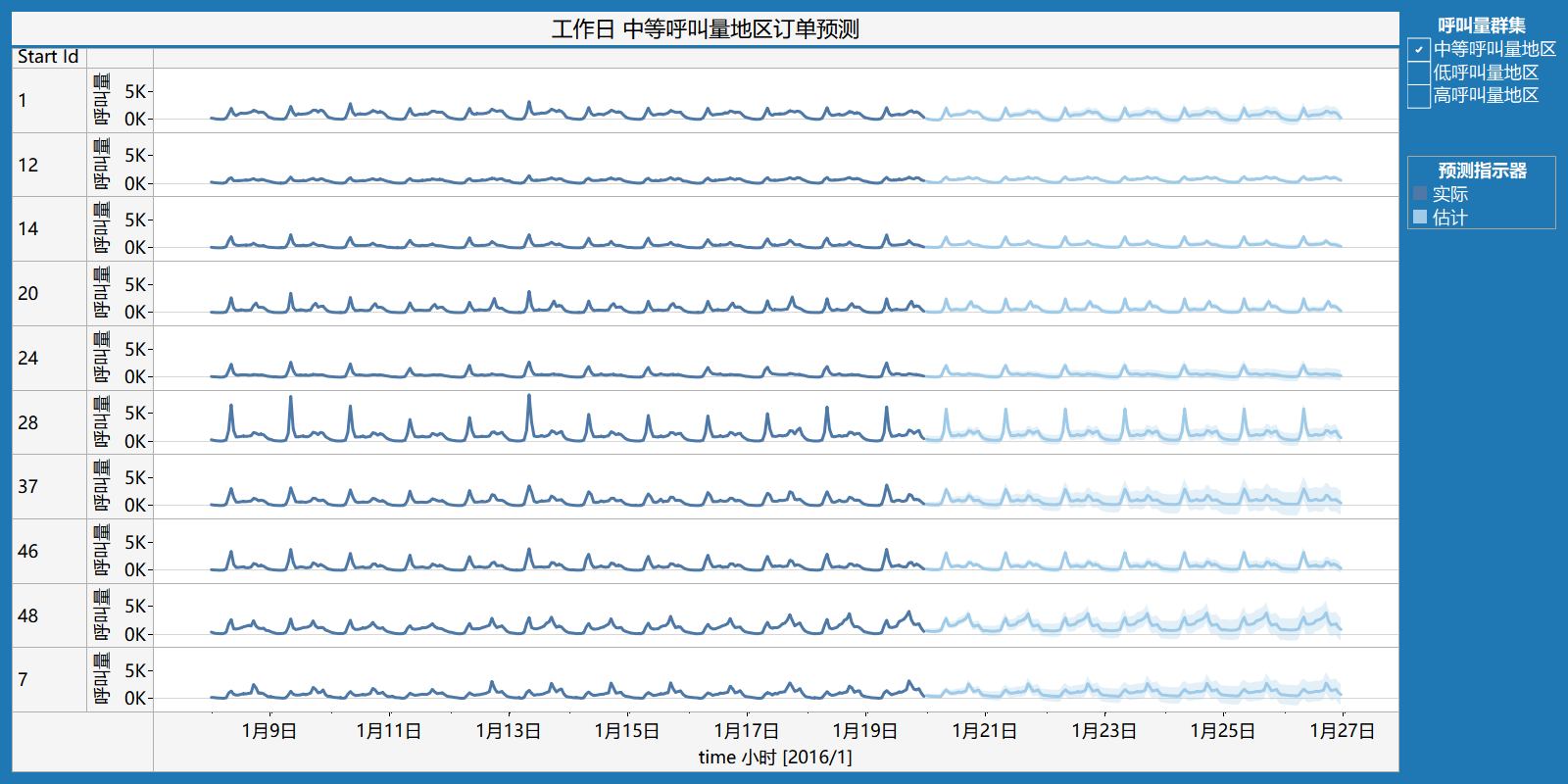
用于创建预测的选项
| 时间序列: | time 小时 |
| 度量: | 呼叫量 |
| 向前预测: | 168 小时 (2016年1月20日 0时 – 2016年1月26日 23时) |
| 预测依据: | 2016年1月8日 0时 – 2016年1月19日 23时 |
| 忽略最后: | 48 小时 (2016年1月20日 0时 – 2016年1月21日 23时) |
| 季节模式: | 24 小时周期 |
工作日(1/22,1/25-1/28)中等呼叫量地区的单量预测和质量评估:
| 行总和 | 初始 | 从初始值更改 | 季节影响 | 贡献 | |||||||
| Start Id | 2016年1月20日 0时 | 2016年1月20日 0时 – 2016年1月26日 23时 | 高 | 低 | 趋势 | 季节 | 质量 | ||||
| 1 | 171 | ± | 199 | 126 | 2016年1月26日 8时 | 1,300 | 2016年1月26日 4时 | -838 | 0.0% | 100.0% | 良好 |
| 12 | 395 | ± | 107 | 169 | 2016年1月26日 8时 | 525 | 2016年1月26日 4时 | -498 | 0.5% | 99.5% | 良好 |
| 14 | 151 | ± | 201 | 98 | 2016年1月26日 8时 | 1,402 | 2016年1月26日 3时 | -460 | 0.1% | 99.9% | 良好 |
| 20 | 157 | ± | 345 | 149 | 2016年1月26日 8时 | 1,783 | 2016年1月26日 3时 | -592 | 0.0% | 100.0% | 良好 |
| 24 | 141 | ± | 210 | 127 | 2016年1月26日 8时 | 1,609 | 2016年1月26日 4时 | -427 | 0.1% | 99.9% | 良好 |
| 28 | 345 | ± | 691 | 271 | 2016年1月26日 8时 | 4,582 | 2016年1月26日 4时 | -1,034 | 0.0% | 100.0% | 良好 |
| 37 | 247 | ± | 338 | 220 | 2016年1月26日 8时 | 2,000 | 2016年1月26日 4时 | -734 | 0.3% | 99.7% | 良好 |
| 46 | 221 | ± | 287 | 159 | 2016年1月26日 8时 | 2,333 | 2016年1月26日 4时 | -672 | 0.2% | 99.8% | 良好 |
| 48 | 616 | ± | 371 | 214 | 2016年1月26日 17时 | 2,081 | 2016年1月26日 3时 | -1,044 | 0.9% | 99.1% | 良好 |
| 7 | 537 | ± | 286 | 189 | 2016年1月26日 17时 | 1,572 | 2016年1月26日 5时 | -688 | 0.8% | 99.2% | 良好 |
drop table if exists order_weekend;
create table order_weekend as(
select
order_id
,start_id
,time
from order_data
where date_format(time,'%w') in (0,6)
)

update order_weekend set time = replace(time,'2016-01-17','2016-01-22')
where DATE_FORMAT(time,'%Y-%m-%d') < '2026-02-01';
update order_weekend set time = replace(time,'2016-01-16','2016-01-21')
where DATE_FORMAT(time,'%Y-%m-%d') < '2026-02-01';
update order_weekend set time = replace(time,'2016-01-10','2016-01-20')
where DATE_FORMAT(time,'%Y-%m-%d') < '2026-02-01';
update order_weekend set time = replace(time,'2016-01-09','2016-01-19')
where DATE_FORMAT(time,'%Y-%m-%d') < '2026-02-01';
update order_weekend set time = replace(time,'2016-01-03','2016-01-18')
where DATE_FORMAT(time,'%Y-%m-%d') < '2026-02-01';
update order_weekend set time = replace(time,'2016-01-02','2016-01-17')
where DATE_FORMAT(time,'%Y-%m-%d') < '2026-02-01';
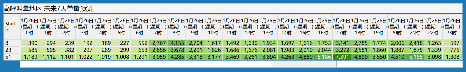
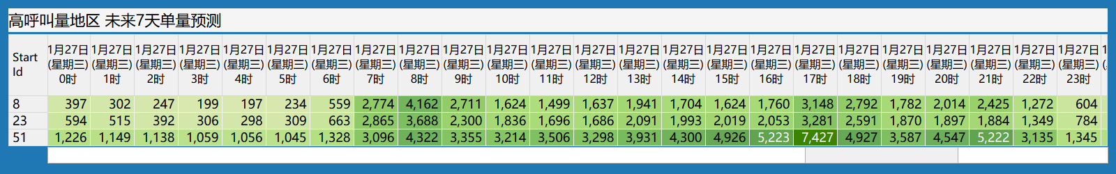
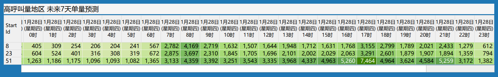
5.3.4 未来7天高呼叫量地区24小时各时段单量预测表:
基于预测需求,可进行调整
1. 提前部署运力
-
每晚生成次日运力地图:将车辆提前部署到预测高需求区域;
-
热点区域标记:识别未来24小时需求高峰时段和区域;
-
潮汐流预调度:工作日保障通勤潮汐流,早7-9点住宅区重兵部署,晚高峰反向调度;周末商圈/景点增派车辆,延长夜间运营;雨雪天气动态调整运力和价格;大型活动结束前1小时周边部署,结束后启动拼车优先。
2. 动态调整(小时级)
-
每60分钟检查预测准确率:对比预测vs实际需求;
-
偏差>15%时:立即从邻近区域调车补缺;
-
运力缓冲池:保留10%车辆应对突发需求。
3. 价格策略
-
预测高需求区:提前小幅涨价(1.1-1.3倍);
-
预测低需求区:提供折扣(0.8-0.9倍);
-
调度激励:对前往预测热点车辆给予补贴。

 浙公网安备 33010602011771号