
pytorch深度学习实战:从全连接神经网络到卷积神经网络
 首先介绍了卷积相对于全连接的三大优势:局部操作、平移不变性和参数量大幅减少。接着讲解了如何通过子类化 nn.Module 自定义模型,重点区分了函数式 API 与模块化 API 的使用场景——有参数的层用模块化,无参数的操作用函数式。最后探讨了三种模型改进策略:增加通道数扩展宽度、使用权重惩罚/Dropout/批量归一化进行正则化、以及通过跳跃连接构建更深的网络以解决梯度消失问题。文末提供了完整的 ResNet 风格网络代码实现。
1. 从全连接到卷积
1.1. 卷积的优势
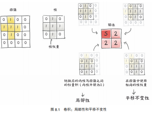
在图像中,卷积对于全连接的优势:
-
局部操作
-
平移不变性
相同的核以及核中的每个权重在整幅图像中被重用。回想一下自动求导,这意味着每个权重的使用都有一个跨越整个图像的历史值。因此,关于卷积权值的损失的导数包括来自整个图像的贡献。
-
模型的参数大幅减少
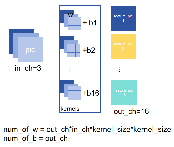
由上得,对于一层网络
卷积权重数量16*3*3*3=1728
全连接权重数量3*32*32=9216
-> 模型参数大幅减小
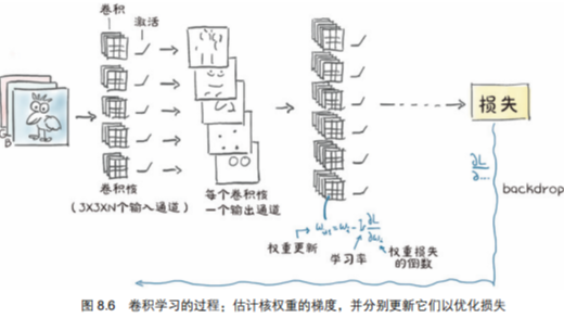
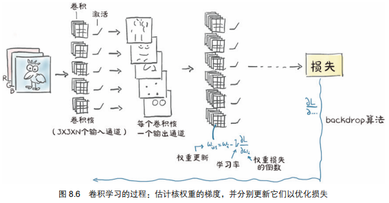
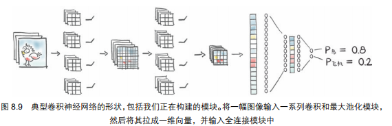
1.2. 卷积神经网络的工作原理
卷积神经网络的工作是估计连续层中的一组过滤器的卷积核,这些过滤器将把一个多通道图像转换成另一个多通道图像,其中不同的通道对应不同的特征,例如一个通道代表平均值,一个通道代表垂直边缘,等等。如下所示
1.3. padding的计算方法
3个关键参数:
| 参数 | 含义 | 常用符号 |
|---|---|---|
| 输入尺寸 | 图像/特征图的边长(比如32×32的图,边长=32) | \(H_{in}\)/\(W_{in}\) |
| 卷积核大小 | 卷积核的边长(比如3×3的核,边长=3) | \(K\) |
| 步长 | 卷积核每次滑动的距离(默认=1) | \(S\) |
则,卷积后输出尺寸的计算公式:
(宽度\(W\)的计算和高度\(H\)完全一样)
import torch.nn as nn

# 方式1:手动指定(3×3卷积核,padding=1,输出尺寸=输入尺寸)
conv = nn.Conv2d(in_channels=3, out_channels=16, kernel_size=3, padding=1, stride=1)

# 方式2:自动计算(PyTorch 1.10+支持,推荐)
conv = nn.Conv2d(in_channels=3, out_channels=16, kernel_size=3, padding="same", stride=1)
1.4. 看到更多特征
如何使用小卷积核看到更大范围(更大的感受野)的物体?
在一个卷积之后堆叠另一个卷积,同时在连续卷积之间对图像进行下采样(池化)。
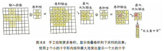
第 1 组卷积核对一阶、低级特征的小邻域进行操作,而第 2 组卷积核则有效地对更宽的邻域进行操作,生成由先前特征组成的特征。
pool = nn.MaxPool2d(2) # 如果我们想把图像缩小一半,我们让核大小为 2
output = pool(img.unsqueeze(0)) # 增加一个 batch 维度
# 32*32 -> 16*16
因此,我们搭建模型:
model = nn.Sequential(
    nn.Conv2d(3, 16, kernel_size=3, padding=1),
    nn.Tanh(),
    nn.MaxPool2d(2),
    nn.Conv2d(16, 8, kernel_size=3, padding=1),
    nn.Tanh(),
    nn.MaxPool2d(2),
    # --- 这里原代码缺少了 Flatten 层 ---
    nn.Linear(8 * 8 * 8, 32),
    nn.Tanh(),
    nn.Linear(32, 2),
)
2. 自定义模型
然而,当我们想要构建模型来做更复杂的事情,而不仅仅是一层接着一层地应用时,我们需要放弃nn.Sequential 运算带来的灵活性。PyTorch 允许我们在模型中通过子类化 nn.Module 来进行任何运算。
- 至少需要定义一个
forward()方法,接收模块的输入并返回输出。 - 为了包含这些子模块,我们通常在构造函数
__init__()中定义运算使用的其他模块,例如内置的卷积或自定义的模块,并将它们分配给 self 以便在 forward()方法中使用。同时,它们将在模块的整个生命周期中保存它们的参数。
PyTorch 如何自动跟踪子模块和参数
2.1. PyTorch 如何自动跟踪子模块和参数
PyTorch 里的 nn.Module 有一个非常聪明的机制:
- 当你在自定义模型的
__init__函数里,把nn.Conv2d、nn.Linear等层赋值为模型的顶级属性时(比如self.conv1 = nn.Conv2d(...)),PyTorch 会自动把这些层识别为“子模块”。 - 这些子模块的参数(权重、偏置)会被自动收集到模型的
parameters()方法里,优化器可以直接通过model.parameters()获取所有可训练参数。
通俗类比
这就像你开了一家公司(模型),招聘了几个部门经理(子模块,如卷积层、全连接层)。公司会自动把所有经理的员工(参数)都纳入人事系统,你不需要一个个去登记。
2.1.1. 为什么子模块不能藏在列表或字典里
如果你把层放在普通的 list 或 dict 里,比如:
self.layers = [nn.Conv2d(...), nn.Linear(...)] # 不能这样写!
PyTorch 就无法自动识别这些子模块,它们的参数也不会被 model.parameters() 收集到,优化器就无法更新这些参数。
解决方法
- 用 PyTorch 提供的
nn.ModuleList或nn.ModuleDict来存放子模块,这样 PyTorch 就能正确跟踪它们。
2.1.2. parameters() 方法的作用
model.parameters() 会递归遍历所有子模块,把所有可训练参数(权重、偏置)收集成一个列表。
比如你定义了一个 ResNet 模型,调用 model.parameters() 会返回所有卷积层、全连接层的权重和偏置。优化器就是通过这个列表来更新模型参数的。
2.1.3. 为什么 forward 里直接调用 nn.ReLU() 不好
如果你在 forward 里直接写:
def forward(self, x):
    x = nn.ReLU()(x)  # 直接调用,没有注册为子模块
    return x
这样的层没有被注册为模型的子模块,而是每次 forward 时临时创建的。
- 这些层如果没有可训练参数(比如
ReLU、MaxPool2d),不会影响参数更新,但会让模型的结构变得不清晰。 - 如果是有参数的层(比如
Conv2d),它们的参数不会被model.parameters()收集,导致优化器无法更新。
正确做法
把所有层都在 __init__ 里注册为子模块,即使是没有参数的层:
def __init__(self):
    self.relu = nn.ReLU()

def forward(self, x):
    x = self.relu(x)
    return x
或者用函数式API,见下节2.2
2.1.4. 总结
- 子模块注册规则:在
__init__里把层赋值为模型的顶级属性(如self.conv1),PyTorch 会自动跟踪。 - 禁止藏在普通容器:不要用普通
list/dict存子模块,要用nn.ModuleList/nn.ModuleDict。 parameters()的作用:自动收集所有子模块的可训练参数,供优化器使用。forward里的层也要注册:即使是无参数层(如ReLU),也建议在__init__里注册,让模型结构更清晰。
2.2. 函数式 API 和模块化 API 的区别以及各自的用法
2.2.1. 什么是函数式 API?
在 PyTorch 里,函数式 API 就是 torch.nn.functional 下的一系列函数(比如 F.linear、F.tanh、F.max_pool2d)。
- 它们没有内部状态,输出完全由输入参数决定。
- 比如
F.linear(input, weight, bias),权重和偏置都需要你手动传进去,函数本身不会保存这些参数。 - 这和
nn.Linear(模块化 API)完全不同:nn.Linear会把权重和偏置作为自己的内部参数保存下来。
通俗类比
- 函数式 API 就像“一次性计算器”:每次计算都要把所有数字(输入、权重、偏置)都给它,算完就扔,不保留任何数据。
- 模块化 API 就像“带记忆的计算器”:会把常用的数字(权重、偏置)存起来,下次直接用,不用每次都重新输入。
2.2.2. 什么时候用函数式 API?
函数式 API 适合那些不需要保存参数和状态的操作,比如:
- 激活函数:
F.tanh、F.relu - 池化操作:
F.max_pool2d - 损失函数:
F.cross_entropy
因为这些操作没有可训练的参数,用函数式 API 更轻量、更灵活。
例子对比
# 模块化 API(有参数,保存权重)
linear_layer = nn.Linear(10, 2)
output = linear_layer(input)

# 函数式 API(无参数,手动传权重)
weight = torch.randn(2, 10)
bias = torch.randn(2)
output = F.linear(input, weight, bias)
2.2.3. 为什么 nn.Linear 和 nn.Conv2d 要用模块化 API?
因为这些层有可训练的参数(权重、偏置),需要在训练中不断更新。
- 模块化 API 会自动保存这些参数,并且通过
model.parameters()让优化器可以轻松找到它们。 - 如果用函数式 API,你需要自己手动管理权重和偏置的更新,非常麻烦。
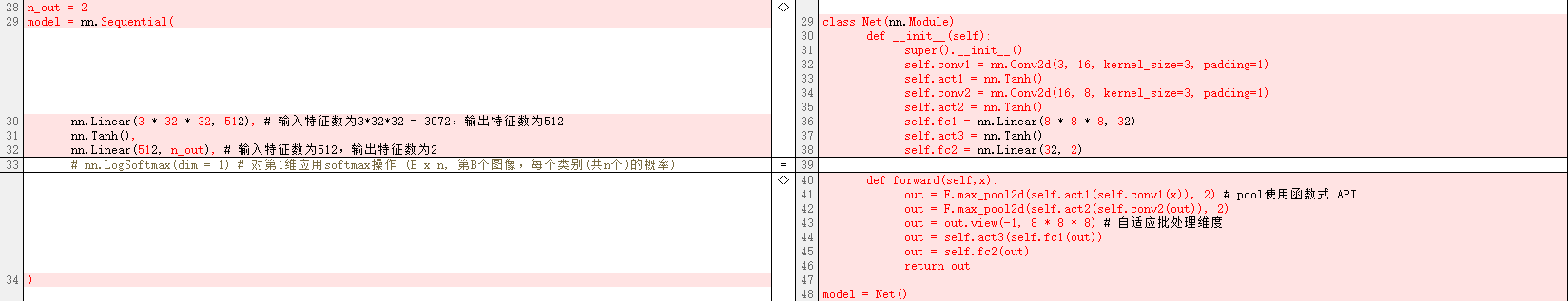
2.2.4. 代码的核心逻辑
你看到的 Net 类就是一个典型的混合使用方式:
class Net(nn.Module):
    def __init__(self):
        super().__init__()
        # 有参数的层用模块化 API
        self.conv1 = nn.Conv2d(3, 16, kernel_size=3, padding=1)
        self.conv2 = nn.Conv2d(16, 8, kernel_size=3, padding=1)
        self.fc1 = nn.Linear(8 * 8 * 8, 32)
        self.fc2 = nn.Linear(32, 2)

    def forward(self, x):
        # 无参数的操作(激活、池化)用函数式 API
        out = F.max_pool2d(torch.tanh(self.conv1(x)), 2) # pool使用函数式 API
        out = F.max_pool2d(torch.tanh(self.conv2(out)), 2)
        out = out.view(-1, 8 * 8 * 8)  # 自适应批处理维度
        out = torch.tanh(self.fc1(out))
        out = self.fc2(out)
        return out
__init__里:用模块化 API 定义有参数的层(卷积、全连接),让 PyTorch 自动跟踪参数。forward里:用函数式 API 处理无参数的操作(tanh、max_pool2d),让代码更简洁。
2.2.5. 为什么说“在 forward 里用 nn.ReLU() 不好”?(接2.1.3.)
如果在 forward 里直接写 nn.ReLU()(x),相当于每次前向传播都创建一个新的 ReLU 实例,既浪费资源,又让模型结构不清晰。
- 正确做法:无参数层也建议在
__init__里注册为子模块(比如self.relu = nn.ReLU()),或者直接用函数式 API(F.relu(x))。
2.2.6. 总结
| 类型 | 优点 | 适用场景 |
|---|---|---|
模块化 API(nn.Linear、nn.Conv2d) |
自动保存参数,优化器可直接获取 | 有可训练参数的层(卷积、全连接) |
函数式 API(F.linear、F.tanh) |
轻量、灵活,无内部状态 | 无参数的操作(激活、池化、损失计算) |
简单来说:有参数的用模块化,没参数的用函数式,这样代码既清晰又高效。
2.3. 最终搭建的模型
在全连接网络的基础上,修改代码为卷积网络。修改部分如下:
点击查看完整代码
import torch
import torch.nn as nn
import torch.optim as optim
from torchvision import datasets
from torchvision.transforms import ToTensor # PIL (0~255) -> Tensor (0.0~1.0)
from torchvision.transforms import Normalize # 归一化
from torchvision.transforms import Compose # 组合多个变换
import torch.nn.functional as F # 函数式 API
# -----------------------------------------------------------------------
# 加载数据
data_path = './data/CIFAR-10/'
transform = Compose([ToTensor(), Normalize((0.4914, 0.4822, 0.4465), (0.2470, 0.2435, 0.2616))])
transformed_cifar10 = datasets.CIFAR10(data_path, train = True, download = True, transform = transform)
transformed_cifar10_val = datasets.CIFAR10(data_path, train = False, download = True, transform = transform)
# -----------------------------------------------------------------------
# 一个只有鸟和飞机的字数据集
label_map = {0: 0, 2: 1} # 0: 鸟, 1: 飞机
class_names = ['airplane', 'bird']
cifar2 = [(img, label_map[label]) for img, label in transformed_cifar10 if label in [0, 2]]
cifar2_val = [(img, label_map[label]) for img, label in transformed_cifar10_val if label in [0, 2]]
train_loader = torch.utils.data.DataLoader(cifar2, batch_size = 64, shuffle = True)
val_loader = torch.utils.data.DataLoader(cifar2_val, batch_size = 64, shuffle = False)
# -----------------------------------------------------------------------
# 搭建一个全连接网络
## 定义模型
class Net(nn.Module):
def __init__(self):
super().__init__()
self.conv1 = nn.Conv2d(3, 16, kernel_size=3, padding=1)
self.act1 = nn.Tanh()
self.conv2 = nn.Conv2d(16, 8, kernel_size=3, padding=1)
self.act2 = nn.Tanh()
self.fc1 = nn.Linear(8 * 8 * 8, 32)
self.act3 = nn.Tanh()
self.fc2 = nn.Linear(32, 2)
def forward(self,x):
out = F.max_pool2d(self.act1(self.conv1(x)), 2) # pool使用函数式 API
out = F.max_pool2d(self.act2(self.conv2(out)), 2)
out = out.view(-1, 8 * 8 * 8) # 自适应批处理维度
out = self.act3(self.fc1(out))
out = self.fc2(out)
return out
model = Net()
learning_rate = 1e-2
optimizer = optim.SGD(model.parameters(), lr = learning_rate)
loss_fn = nn.CrossEntropyLoss()
# -----------------------------------------------------------------------
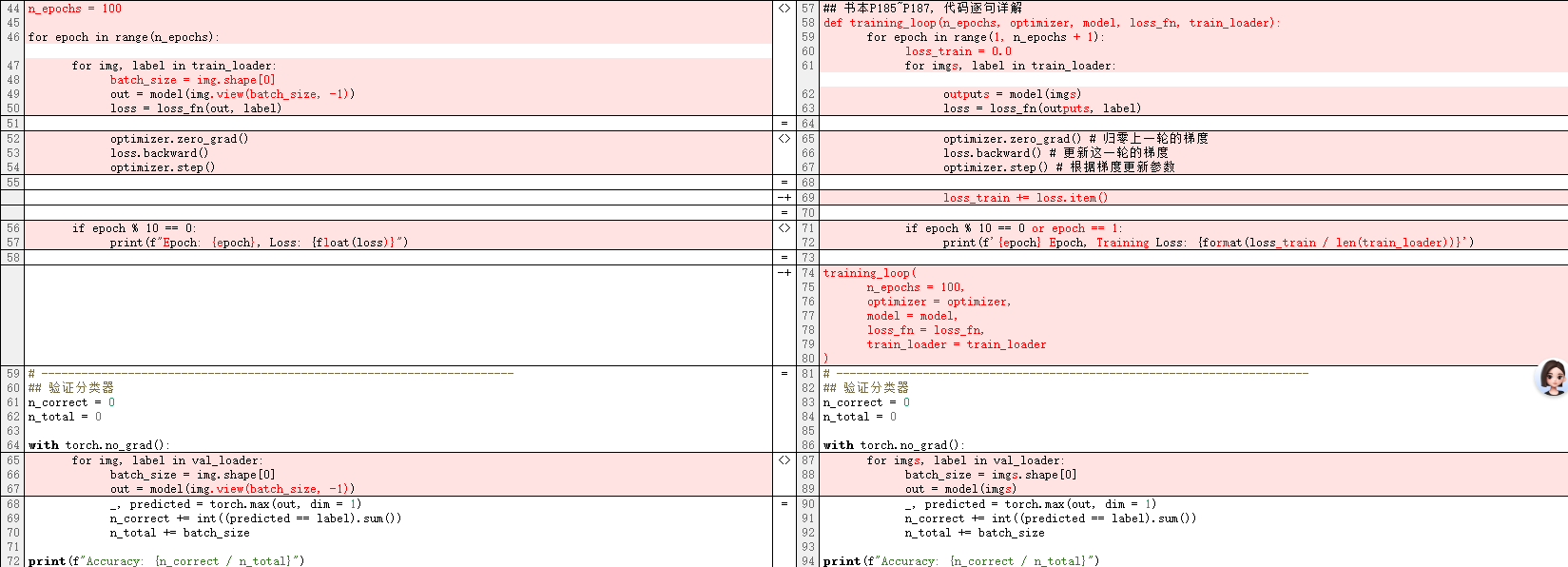
## 训练分类器
## 书本P185~P187, 代码逐句详解
def training_loop(n_epochs, optimizer, model, loss_fn, train_loader):
for epoch in range(1, n_epochs + 1):
loss_train = 0.0
for imgs, label in train_loader:
outputs = model(imgs)
loss = loss_fn(outputs, label)
optimizer.zero_grad() # 归零上一轮的梯度
loss.backward() # 更新这一轮的梯度
optimizer.step() # 根据梯度更新参数
loss_train += loss.item()
if epoch % 10 == 0 or epoch == 1:
print(f'{epoch} Epoch, Training Loss: {format(loss_train / len(train_loader))}')
training_loop(
n_epochs = 100,
optimizer = optimizer,
model = model,
loss_fn = loss_fn,
train_loader = train_loader
)
# -----------------------------------------------------------------------
## 验证分类器
def validate(model, train_loader, val_loader):
for name, loader in [("train", train_loader), ("val", val_loader)]:
n_correct = 0
n_total = 0
with torch.no_grad():
for imgs, label in loader:
out = model(imgs)
_, predicted = torch.max(out, dim = 1)
n_correct += int((predicted == label).sum())
n_total += imgs.shape[0]
print(f"{name} Accuracy: {n_correct / n_total}")
validate(model, train_loader, val_loader)
输出:
1 Epoch, Training Loss: 0.5591110106866071
10 Epoch, Training Loss: 0.3240322130880538
20 Epoch, Training Loss: 0.28498813206223167
30 Epoch, Training Loss: 0.26027746427400855
40 Epoch, Training Loss: 0.24314728122987564
50 Epoch, Training Loss: 0.23136532102610655
60 Epoch, Training Loss: 0.218075687433504
70 Epoch, Training Loss: 0.20048291872071614
80 Epoch, Training Loss: 0.19081769541949983
90 Epoch, Training Loss: 0.17507808528555807
100 Epoch, Training Loss: 0.1622462912349944
train Accuracy: 0.9368
val Accuracy: 0.8995
2.4. GPU 训练
在GPU训练, 需要修改如下部分:
# 检查GPU设备
# -----------------------------------------------------------------------
# 选择设备
device = torch.device('cuda' if torch.cuda.is_available() else 'cpu')
print(f'Using device: {device}')

# -----------------------------------------------------------------------
# 将模型移动到GPU
model = Net().to(device=device)# <- GPU

# -----------------------------------------------------------------------
# 将dataloader中的内容移动到cpu
def training_loop(n_epochs, optimizer, model, loss_fn, train_loader):
    for epoch in range(1, n_epochs + 1):
        loss_train = 0.0
        for imgs, label in train_loader:
            imgs = imgs.to(device=device)  # <- GPU
            label = label.to(device=device)
            # ...

# -----------------------------------------------------------------------
## 验证分类器
def validate(model, train_loader, val_loader):
    for name, loader in [("train", train_loader), ("val", val_loader)]:
        n_correct = 0
        n_total = 0

        with torch.no_grad():
            for imgs, label in loader:
                imgs = imgs.to(device=device) # <- GPU
                label = label.to(device=device) # <- GPU
2.5. 保存与加载模型
2.5.1. 保存模型
torch.save(model.state_dict(), './data/cifar2_model.pt')
2.5.2. 加载模型
load_model = Net()
load_model.load_state_dict(torch.load('./data/cifar2_model.pt'))
注意当加载权重时,需要指示pytorch覆盖设备信息:
load_model = Net().to(device=device)
load_model.load_state_dict(torch.load('./data/cifar2_model.pt'),
                            map_location=device)  # <- 注意此处
原因:
加载网络权重时有一点儿复杂:PyTorch 将尝试将权重加载到保存它的同一设备上。也就是说,GPU 上的权重将恢复到 GPU 上。由于我们不知道是否需要相同的设备,我们有 2 个选择:在保存之前将网络移动到 CPU,或者在恢复后将其移回。在加载权重时,指示 PyTorch 覆盖设备信息会更简洁一些。这是通过将 map_location 关键字参数传递给 torch.load 来实现的
3. 改进模型
3.1. 增加内存容量:宽度
# 避免模型中的硬编码
class Net(nn.Module):
    def __init__(self, n_chans1 = 32): # 16 -> 32 增加内存容量:宽度,但是容易过拟合
        super().__init__()
        self.conv1 = nn.Conv2d(3, n_chans1, kernel_size=3, padding=1)
        self.act1 = nn.Tanh()
        self.conv2 = nn.Conv2d(n_chans1, n_chans1 // 2, kernel_size=3, padding=1)
        self.act2 = nn.Tanh()
        self.fc1 = nn.Linear(8 * 8 * n_chans1 // 2, 32)
        self.act3 = nn.Tanh()
        self.fc2 = nn.Linear(32, 2)

    def forward(self,x):
        out = F.max_pool2d(self.act1(self.conv1(x)), 2) # pool使用函数式 API
        out = F.max_pool2d(self.act2(self.conv2(out)), 2)
        out = out.view(-1, 8 * 8 * n_chans1 // 2) # 自适应批处理维度
        out = self.act3(self.fc1(out))
        out = self.fc2(out)
        return out
3.2. 帮助模型收敛和泛化:正则化
训练模型涉及 2 个关键步骤:一是优化,当我们需要减少训练集上的损失时;二是泛化,当模型不仅要处理训练集,还要处理以前没有见过的数据,如验证集时。旨在简化这 2 个步骤的数学工具有时被归入正则化的标签之下。
3.2.1. 检查参数:权重惩罚
作用:稳定泛化,防止过拟合。
避免关注几个特征,让模型更关注通用特征。
给模型加 “紧箍咒”,参数不能变得太大(避免过拟合)。
# weight_decay实现
optimizer2 = optim.SGD(model.parameters(), lr=0.01, weight_decay=1e-4)  # λ=1e-4
3.2.2. 不太依赖单一输入:Dropout
作用:防止过拟合
将网络每轮训练迭代中的神经元随机部分清零。
在 PyTorch 中,我们可以通过在非线性激活与后面的线性或卷积模块之间添加一个nn.Dropout 模块在模型中实现 Dropout。作为一个参数,我们需要指定输入归零的概率。如果是卷积,我们将使用专门的 nn.Dropout2d 或者 nn.Dropout3d,将输入的所有通道归零.
需要区分model.train()和model.eval()
class Net(nn.Module):
    def __init__(self, n_chans1 = 32):
        super().__init__()
        self.conv1 = nn.Conv2d(3, n_chans1, kernel_size=3, padding=1)
        self.conv1_dropout = nn.Dropout2d(p=0.4)
        self.conv2 = nn.Conv2d(n_chans1, n_chans1 // 2, kernel_size=3, padding=1)
        self.conv2_dropout = nn.Dropout2d(p=0.4)
        self.fc1 = nn.Linear(8 * 8 * n_chans1 // 2, 32)
        self.fc2 = nn.Linear(32, 2)

    def forward(self,x):
        out = F.max_pool2d(torch.tanh(self.conv1(x)), 2)
        out = self.conv1_dropout(out)
        out = F.max_pool2d(torch.tanh(self.conv2(out)), 2)
        out = self.conv2_dropout(out)
        out = out.view(-1, 8 * 8 * n_chans1 // 2)
        out = torch.tanh(self.fc1(out))
        out = self.fc2(out)
        return out
3.2.3. 保存激活检查:批量归一化
作用:提高学习率,减少训练对初始化的依赖,并充当正则化器,提出了一种替代 Dropout 的方法。主要思想是将输入重新调整到网络的激活状态,从而使小批量具有一定的理想分布。
需要区分model.train()和model.eval()
class NetBatchNorm(nn.Module):
    def __init__(self, n_chans1=32):
        super().__init__()
        self.n_chans1 = n_chans1
        self.conv1 = nn.Conv2d(3, n_chans1, kernel_size=3, padding=1)
        self.conv1_batchnorm = nn.BatchNorm2d(num_features=n_chans1)
        self.conv2 = nn.Conv2d(n_chans1, n_chans1 // 2, kernel_size=3,
        padding=1)
        self.conv2_batchnorm = nn.BatchNorm2d(num_features=n_chans1 // 2)
        self.fc1 = nn.Linear(8 * 8 * n_chans1 // 2, 32)
        self.fc2 = nn.Linear(32, 2)

    def forward(self, x):
        out = self.conv1_batchnorm(self.conv1(x))
        out = F.max_pool2d(torch.tanh(out), 2)
        out = self.conv2_batchnorm(self.conv2(out))
        out = F.max_pool2d(torch.tanh(out), 2)
        out = out.view(-1, 8 * 8 * self.n_chans1 // 2)
        out = torch.tanh(self.fc1(out))
        out = self.fc2(out)
        return out
3.3. 更复杂的结构:深度
3.3.1. 跳跃连接
深度带来挑战:
1.梯度消失/爆炸。反向传播的梯度会在逐层传递中不断缩小,导致浅层的参数几乎无法更新。
2.参数数量增加,容易过拟合
跳跃连接在反向传播时,梯度可以通过跳跃连接直接传递到浅层:
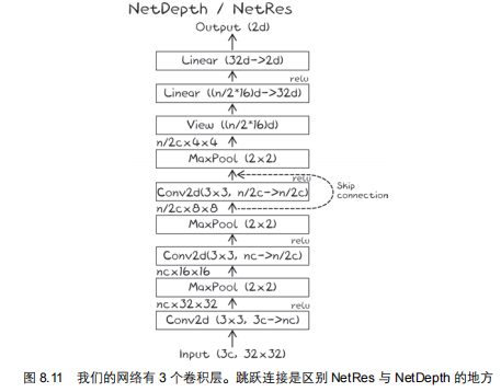
class NetRes(nn.Module):
    def __init__(self, n_chans1=32):
        super().__init__()
        self.n_chans1 = n_chans1
        self.conv1 = nn.Conv2d(3, n_chans1, kernel_size=3, padding=1)
        self.conv2 = nn.Conv2d(n_chans1, n_chans1 // 2, kernel_size=3,
        padding=1)
        self.conv3 = nn.Conv2d(n_chans1 // 2, n_chans1 // 2,
        kernel_size=3, padding=1)
        self.fc1 = nn.Linear(4 * 4 * n_chans1 // 2, 32)
        self.fc2 = nn.Linear(32, 2)

    def forward(self, x):
        out = F.max_pool2d(torch.relu(self.conv1(x)), 2)
        out = F.max_pool2d(torch.relu(self.conv2(out)), 2)
        out1 = out
        out = F.max_pool2d(torch.relu(self.conv3(out)) + out1, 2)
        out = out.view(-1, 4 * 4 * self.n_chans1 // 2)
        out = torch.relu(self.fc1(out))
        out = self.fc2(out)
        return out
3.3.2. 用跳跃连接建立一个非常深的模型
接着,我们可以用跳跃连接建立一个非常深的模型:
# 模块子类,为一个块提供运算,
class ResBlock(nn.Module):
    def __init__(self, n_chans):
        super().__init__()
        self.conv = nn.Conv2d(n_chans, n_chans, kernel_size=3, padding=1, bias=False)
        self.batch_norm = nn.BatchNorm2d(num_features=n_chans)
        torch.nn.init.kaiming_normal_(self.conv.weight, nonlinearity='relu')
        torch.nn.init.constant_(self.batch_norm.weight, 0.5)
        torch.nn.init.zeros_(self.batch_norm.bias)

    def forward(self, x):
        out = self.conv(x)
        out = self.batch_norm(out)
        out = torch.relu(out)
        return out + x

# 网络模型
class Net(nn.Module):
    def __init__(self, n_chans1=32, n_blocks=10):
        super().__init__()
        self.n_chans1 = n_chans1
        self.conv1 = nn.Conv2d(3, n_chans1, kernel_size=3, padding=1)

        # - ResBlock(n_chans=n_chans1):创建一个残差块实例(比如通道数为 32 的 ResBlock);
        # - [ResBlock(...)]:把这一个实例放进列表,得到 [ResBlock实例];
        # - n_blocks * [...]:把列表重复 n_blocks 次(比如 n_blocks=10 时,得到包含 10 个 ResBlock 实例的列表 [ResBlock, ResBlock, ..., ResBlock])
        # - *:解包列表,把列表元素变成 nn.Sequential 的独立参数
        self.resblocks = nn.Sequential(
        *(n_blocks * [ResBlock(n_chans=n_chans1)]))  # <-

        self.fc1 = nn.Linear(8 * 8 * n_chans1, 32)
        self.fc2 = nn.Linear(32, 2)
    def forward(self, x):
        out = F.max_pool2d(torch.relu(self.conv1(x)), 2)
        out = self.resblocks(out)  # <-
        out = F.max_pool2d(out, 2)
        out = out.view(-1, 8 * 8 * self.n_chans1)
        out = torch.relu(self.fc1(out))
        out = self.fc2(out)
        return out
4. 本文最终代码
点击展开
# 更深的卷积网络(利用跳跃连接)
import torch
import torch.nn as nn
import torch.optim as optim
from torchvision import datasets
from torchvision.transforms import ToTensor # PIL (0~255) -> Tensor (0.0~1.0)
from torchvision.transforms import Normalize # 归一化
from torchvision.transforms import Compose # 组合多个变换
import torch.nn.functional as F # 函数式 API

# -----------------------------------------------------------------------
# 加载数据
data_path = './data/CIFAR-10/'
transform = Compose([ToTensor(), Normalize((0.4914, 0.4822, 0.4465), (0.2470, 0.2435, 0.2616))])
transformed_cifar10 = datasets.CIFAR10(data_path, train = True, download = True, transform = transform)
transformed_cifar10_val = datasets.CIFAR10(data_path, train = False, download = True, transform = transform)

# -----------------------------------------------------------------------
# 一个只有鸟和飞机的字数据集
label_map = {0: 0, 2: 1} # 0: 鸟, 1: 飞机
class_names = ['airplane', 'bird']
cifar2 = [(img, label_map[label]) for img, label in transformed_cifar10 if label in [0, 2]]
cifar2_val = [(img, label_map[label]) for img, label in transformed_cifar10_val if label in [0, 2]]

train_loader = torch.utils.data.DataLoader(cifar2, batch_size = 64, shuffle = True)
val_loader = torch.utils.data.DataLoader(cifar2_val, batch_size = 64, shuffle = False)

# -----------------------------------------------------------------------
# 选择设备
device = torch.device('cuda' if torch.cuda.is_available() else 'cpu')
print(f'Using device: {device}')

# -----------------------------------------------------------------------
# 搭建一个全连接网络
## 定义模型
class ResBlock(nn.Module):
    def __init__(self, n_chans):
        super().__init__()
        self.conv = nn.Conv2d(n_chans, n_chans, kernel_size=3, padding=1, bias=False)
        self.batch_norm = nn.BatchNorm2d(num_features=n_chans)
        torch.nn.init.kaiming_normal_(self.conv.weight, nonlinearity='relu')
        torch.nn.init.constant_(self.batch_norm.weight, 0.5)
        torch.nn.init.zeros_(self.batch_norm.bias)

    def forward(self, x):
        out = self.conv(x)
        out = self.batch_norm(out)
        out = torch.relu(out)
        return out + x

class Net(nn.Module):
    def __init__(self, n_chans1=32, n_blocks=10):
        super().__init__()
        self.n_chans1 = n_chans1
        self.conv1 = nn.Conv2d(3, n_chans1, kernel_size=3, padding=1)
        self.resblocks = nn.Sequential(
        *(n_blocks * [ResBlock(n_chans=n_chans1)]))
        self.fc1 = nn.Linear(8 * 8 * n_chans1, 32)
        self.fc2 = nn.Linear(32, 2)
    def forward(self, x):
        out = F.max_pool2d(torch.relu(self.conv1(x)), 2)
        out = self.resblocks(out)
        out = F.max_pool2d(out, 2)
        out = out.view(-1, 8 * 8 * self.n_chans1)
        out = torch.relu(self.fc1(out))
        out = self.fc2(out)
        return out

model = Net().to(device=device)
model.parameters()
for p in model.parameters():
    print(p.shape)
    p.numel()

learning_rate = 3e-3
optimizer = optim.SGD(model.parameters(), lr = learning_rate)

loss_fn = nn.CrossEntropyLoss()

# -----------------------------------------------------------------------
## 训练分类器
## 书本P185~P187, 代码逐句详解
def training_loop(n_epochs, optimizer, model, loss_fn, train_loader):
    for epoch in range(1, n_epochs + 1):
        loss_train = 0.0
        for imgs, label in train_loader:
            imgs = imgs.to(device=device)
            label = label.to(device=device)
            outputs = model(imgs)
            loss = loss_fn(outputs, label)

            optimizer.zero_grad() # 归零上一轮的梯度
            loss.backward() # 更新这一轮的梯度
            optimizer.step() # 根据梯度更新参数

            loss_train += loss.item()

        if epoch % 10 == 0 or epoch == 1:
            print(f'{epoch} Epoch, Training Loss: {format(loss_train / len(train_loader))}')

training_loop(
    n_epochs = 100,
    optimizer = optimizer,
    model = model,
    loss_fn = loss_fn,
    train_loader = train_loader
)
# -----------------------------------------------------------------------
## 验证分类器
def validate(model, train_loader, val_loader):
    for name, loader in [("train", train_loader), ("val", val_loader)]:
        n_correct = 0
        n_total = 0

        with torch.no_grad():
            for imgs, label in loader:
                imgs = imgs.to(device=device)
                label = label.to(device=device)
                out = model(imgs)
                _, predicted = torch.max(out, dim = 1)
                n_correct += int((predicted == label).sum())
                n_total += imgs.shape[0]

        print(f"{name} Accuracy: {n_correct / n_total}")

validate(model, train_loader, val_loader)
输出:
Using device: cuda
1 Epoch, Training Loss: 0.49166663057485205
10 Epoch, Training Loss: 0.2634233754531593
20 Epoch, Training Loss: 0.1906170040891049
30 Epoch, Training Loss: 0.12040648637873352
40 Epoch, Training Loss: 0.06903127147252583
50 Epoch, Training Loss: 0.03015419604422845
60 Epoch, Training Loss: 0.015214779083528052
70 Epoch, Training Loss: 0.010205398788260427
80 Epoch, Training Loss: 0.005108015554672356
90 Epoch, Training Loss: 0.0037311426546294125
100 Epoch, Training Loss: 0.0026776732909893556
train Accuracy: 1.0
val Accuracy: 0.8835

 浙公网安备 33010602011771号