

Tensorflow2.0进阶学习-RNN生成音频 (十二)
引包
import collections
import datetime
import fluidsynth
import glob
import numpy as np
import pathlib
import pandas as pd
import pretty_midi
import seaborn as sns
import tensorflow as tf

from IPython import display
from matplotlib import pyplot as plt
from typing import Dict, List, Optional, Sequence, Tuple
啰哩啰嗦一大堆,要注意fluidsynth和pretty_midi的安装,可参照网上资料。
数据熟悉
一些预先准备
seed = 42
tf.random.set_seed(seed)
np.random.seed(seed)

# 设定音频的采样率,这里设定为16000
_SAMPLING_RATE = 16000
下载数据
data_dir = pathlib.Path('data/maestro-v2.0.0')
if not data_dir.exists():
  tf.keras.utils.get_file(
      'maestro-v2.0.0-midi.zip',
      origin='https://storage.googleapis.com/magentadata/datasets/maestro/v2.0.0/maestro-v2.0.0-midi.zip',
      extract=True,
      cache_dir='.', cache_subdir='data',
  )
看看下载数据有多大
filenames = glob.glob(str(data_dir/'**/*.mid*'))
print('Number of files:', len(filenames))
# 一共1282个文件
# Number of files: 1282
对MIDI文件进行处理
再看看下载数据格式,是midi格式的文件,这个需要PrettyMIDI库来处理
sample_file = filenames[1]
print(sample_file)

# data/maestro-v2.0.0/2013/ORIG-MIDI_03_7_6_13_Group__MID--AUDIO_09_R1_2013_wav--2.midi
将其定义为pretty_midi实例,方便以后操作
pm = pretty_midi.PrettyMIDI(sample_file)
再定一个方法对数据进行播放,播放时长可以自定义
def display_audio(pm: pretty_midi.PrettyMIDI, seconds=30):
  waveform = pm.fluidsynth(fs=_SAMPLING_RATE)
  # Take a sample of the generated waveform to mitigate kernel resets
  waveform_short = waveform[:seconds*_SAMPLING_RATE]
  return display.Audio(waveform_short, rate=_SAMPLING_RATE)
在jupyter执行下面代码,会出现播放控件,可以播放
display_audio(pm)
pm里除了音乐还有一些音乐介绍
print('Number of instruments:', len(pm.instruments))
instrument = pm.instruments[0]
instrument_name = pretty_midi.program_to_instrument_name(instrument.program)
print('Instrument name:', instrument_name)

# Number of instruments: 1
# Instrument name: Acoustic Grand Piano
数据打印
打印出来的pm可以看成乐谱,有一些音符信息,有音高,有持续时间,还有步长
for i, note in enumerate(instrument.notes[:10]):
  note_name = pretty_midi.note_number_to_name(note.pitch)
  duration = note.end - note.start
  print(f'{i}: pitch={note.pitch}, note_name={note_name},'
        f' duration={duration:.4f}')

0: pitch=75, note_name=D#5, duration=0.0677
1: pitch=63, note_name=D#4, duration=0.0781
2: pitch=75, note_name=D#5, duration=0.0443
3: pitch=63, note_name=D#4, duration=0.0469
4: pitch=75, note_name=D#5, duration=0.0417
5: pitch=63, note_name=D#4, duration=0.0469
6: pitch=87, note_name=D#6, duration=0.0443
7: pitch=99, note_name=D#7, duration=0.0690
8: pitch=87, note_name=D#6, duration=0.0378
9: pitch=99, note_name=D#7, duration=0.0742
将pm信息处理成模型可输入的格式
def midi_to_notes(midi_file: str) -> pd.DataFrame:
pm = pretty_midi.PrettyMIDI(midi_file)
instrument = pm.instruments[0]
notes = collections.defaultdict(list)
# Sort the notes by start time
sorted_notes = sorted(instrument.notes, key=lambda note: note.start)
prev_start = sorted_notes[0].start
for note in sorted_notes:
start = note.start
end = note.end
notes['pitch'].append(note.pitch)
notes['start'].append(start)
notes['end'].append(end)
notes['step'].append(start - prev_start)
notes['duration'].append(end - start)
prev_start = start
return pd.DataFrame({name: np.array(value) for name, value in notes.items()})
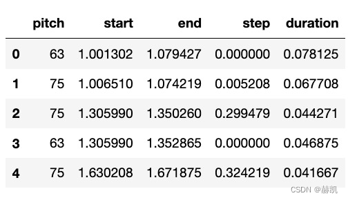
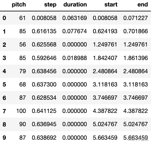
raw_notes = midi_to_notes(sample_file)
raw_notes.head()
也可以看一些音符信息
get_note_names = np.vectorize(pretty_midi.note_number_to_name)
sample_note_names = get_note_names(raw_notes['pitch'])
sample_note_names[:10]

# array(['D#4', 'D#5', 'D#5', 'D#4', 'D#5', 'D#4', 'D#7', 'D#6', 'D#7', 'D#6'], dtype='<U3')
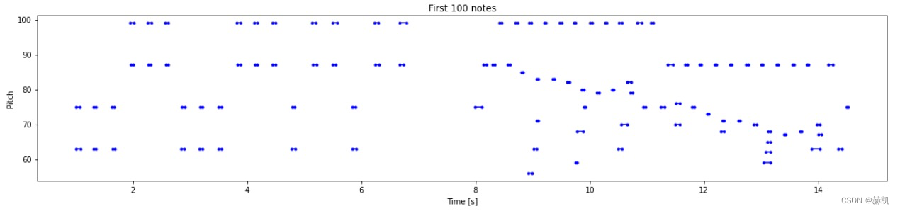
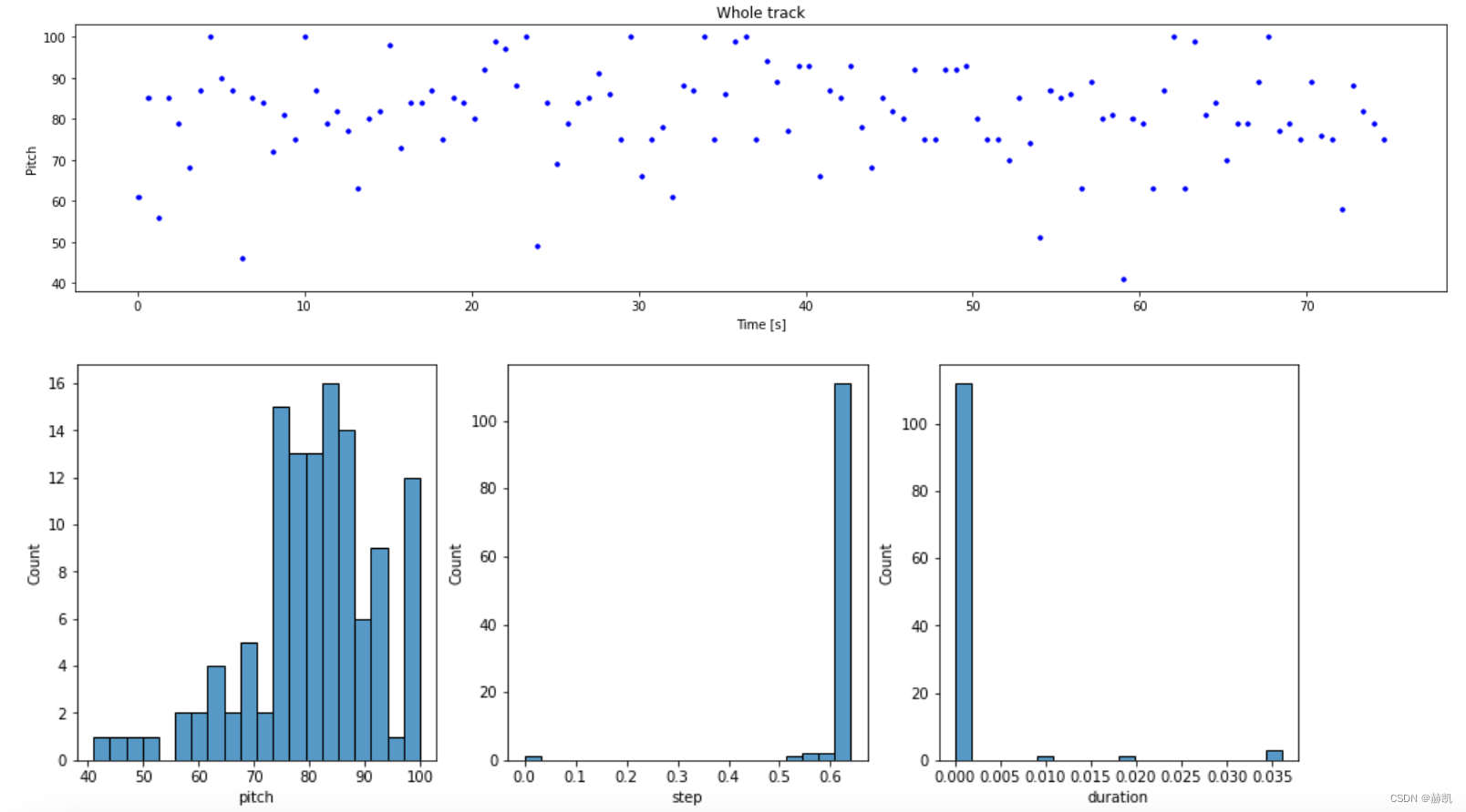
可以用图的形式来表达乐谱
def plot_piano_roll(notes: pd.DataFrame, count: Optional[int] = None):
  if count:
    title = f'First {count} notes'
  else:
    title = f'Whole track'
    count = len(notes['pitch'])
  plt.figure(figsize=(20, 4))
  plot_pitch = np.stack([notes['pitch'], notes['pitch']], axis=0)
  plot_start_stop = np.stack([notes['start'], notes['end']], axis=0)
  plt.plot(
      plot_start_stop[:, :count], plot_pitch[:, :count], color="b", marker=".")
  plt.xlabel('Time [s]')
  plt.ylabel('Pitch')
  _ = plt.title(title)

plot_piano_roll(raw_notes, count=100)
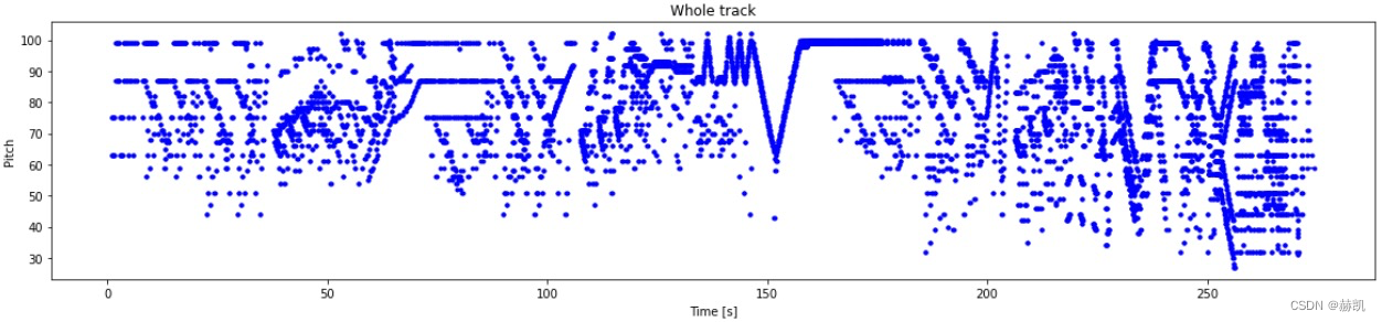
来看下全部的样子
plot_piano_roll(raw_notes)
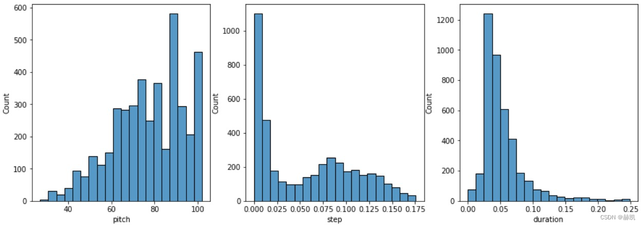
看看他们的直方图
def plot_distributions(notes: pd.DataFrame, drop_percentile=2.5):
  plt.figure(figsize=[15, 5])
  plt.subplot(1, 3, 1)
  sns.histplot(notes, x="pitch", bins=20)

  plt.subplot(1, 3, 2)
  max_step = np.percentile(notes['step'], 100 - drop_percentile)
  sns.histplot(notes, x="step", bins=np.linspace(0, max_step, 21))

  plt.subplot(1, 3, 3)
  max_duration = np.percentile(notes['duration'], 100 - drop_percentile)
  sns.histplot(notes, x="duration", bins=np.linspace(0, max_duration, 21))

plot_distributions(raw_notes)
创造MIDI文件
这个是方法
def notes_to_midi(
  notes: pd.DataFrame,
  out_file: str,
  instrument_name: str,
  velocity: int = 100,  # note loudness
) -> pretty_midi.PrettyMIDI:

  pm = pretty_midi.PrettyMIDI()
  instrument = pretty_midi.Instrument(
      program=pretty_midi.instrument_name_to_program(
          instrument_name))

  prev_start = 0
  for i, note in notes.iterrows():
    start = float(prev_start + note['step'])
    end = float(start + note['duration'])
    note = pretty_midi.Note(
        velocity=velocity,
        pitch=int(note['pitch']),
        start=start,
        end=end,
    )
    instrument.notes.append(note)
    prev_start = start

  pm.instruments.append(instrument)
  pm.write(out_file)
  return pm

# 用上面的note信息试一下
example_file = 'example.midi'
example_pm = notes_to_midi(
    raw_notes, out_file=example_file, instrument_name=instrument_name)

display_audio(example_pm)
两个方法notes_to_midi和midi_to_notes可以将音频转换为模型输入数据,也可将输入数据转换为音频,这里打通了就好说了。
数据准备
先用小数据训练
num_files = 5
all_notes = []
for f in filenames[:num_files]:
  notes = midi_to_notes(f)
  all_notes.append(notes)

all_notes = pd.concat(all_notes)

n_notes = len(all_notes)
print('Number of notes parsed:', n_notes)

# Number of notes parsed: 15435
终于转变为我们喜闻乐见的tf.data.Dataset了
key_order = ['pitch', 'step', 'duration']
train_notes = np.stack([all_notes[key] for key in key_order], axis=1)
notes_ds = tf.data.Dataset.from_tensor_slices(train_notes)
notes_ds.element_spec

# TensorSpec(shape=(3,), dtype=tf.float64, name=None)
既然是RNN,就是用一段连续的数据,预测这段数据接下来的数据,需要维护一个窗口去生成input和label
def create_sequences(
    dataset: tf.data.Dataset,
    seq_length: int,
    vocab_size = 128,
) -> tf.data.Dataset:
  """Returns TF Dataset of sequence and label examples."""
  seq_length = seq_length+1

  # Take 1 extra for the labels
  windows = dataset.window(seq_length, shift=1, stride=1,
                              drop_remainder=True)

  # `flat_map` flattens the" dataset of datasets" into a dataset of tensors
  flatten = lambda x: x.batch(seq_length, drop_remainder=True)
  sequences = windows.flat_map(flatten)

  # Normalize note pitch
  def scale_pitch(x):
    x = x/[vocab_size,1.0,1.0]
    return x

  # Split the labels
  def split_labels(sequences):
    inputs = sequences[:-1]
    labels_dense = sequences[-1]
    labels = {key:labels_dense[i] for i,key in enumerate(key_order)}

    return scale_pitch(inputs), labels

  return sequences.map(split_labels, num_parallel_calls=tf.data.AUTOTUNE)

seq_length = 25
vocab_size = 128
seq_ds = create_sequences(notes_ds, seq_length, vocab_size)
seq_ds.element_spec

# (TensorSpec(shape=(25, 3), dtype=tf.float64, name=None),
# {'pitch': TensorSpec(shape=(), dtype=tf.float64, name=None),
# 'step': TensorSpec(shape=(), dtype=tf.float64, name=None),
# 'duration': TensorSpec(shape=(), dtype=tf.float64, name=None)})
看一个训练数据和标签
for seq, target in seq_ds.take(1):
  print('sequence shape:', seq.shape)
  print('sequence elements (first 10):', seq[0: 10])
  print()
  print('target:', target)

sequence shape: (25, 3)
sequence elements (first 10): tf.Tensor(
[[0.6015625  0.         0.09244792]
 [0.3828125  0.00390625 0.40234375]
 [0.5703125  0.109375   0.06510417]
 [0.53125    0.09895833 0.06119792]
 [0.5703125  0.10807292 0.05989583]
 [0.4765625  0.06640625 0.05338542]
 [0.6015625  0.01302083 0.0703125 ]
 [0.5703125  0.11979167 0.07682292]
 [0.3984375  0.109375   0.43619792]
 [0.609375   0.00130208 0.09505208]], shape=(10, 3), dtype=float64)

target: {'pitch': <tf.Tensor: shape=(), dtype=float64, numpy=54.0>, 'step': <tf.Tensor: shape=(), dtype=float64, numpy=0.005208333333333037>, 'duration': <tf.Tensor: shape=(), dtype=float64, numpy=0.46875>}
用25个数据去预测最后一个数据,每个数据包含音高、步长和持续时间。
真正的训练数据
batch_size = 64
buffer_size = n_notes - seq_length  # the number of items in the dataset
train_ds = (seq_ds
            .shuffle(buffer_size)
            .batch(batch_size, drop_remainder=True)
            .cache()
            .prefetch(tf.data.experimental.AUTOTUNE))

train_ds.element_spec

# (TensorSpec(shape=(64, 25, 3), dtype=tf.float64, name=None),
# {'pitch': TensorSpec(shape=(64,), dtype=tf.float64, name=None),
# 'step': TensorSpec(shape=(64,), dtype=tf.float64, name=None),
# 'duration': TensorSpec(shape=(64,), dtype=tf.float64, name=None)})
模型准备
自定义一个损失函数
def mse_with_positive_pressure(y_true: tf.Tensor, y_pred: tf.Tensor):
  mse = (y_true - y_pred) ** 2
  positive_pressure = 10 * tf.maximum(-y_pred, 0.0)
  return tf.reduce_mean(mse + positive_pressure)
定义输入尺寸、学习率、网络模型。
input_shape = (seq_length, 3)
learning_rate = 0.005

inputs = tf.keras.Input(input_shape)
x = tf.keras.layers.LSTM(128)(inputs)

outputs = {
  'pitch': tf.keras.layers.Dense(128, name='pitch')(x),
  'step': tf.keras.layers.Dense(1, name='step')(x),
  'duration': tf.keras.layers.Dense(1, name='duration')(x),
}

model = tf.keras.Model(inputs, outputs)

loss = {
      'pitch': tf.keras.losses.SparseCategoricalCrossentropy(
          from_logits=True),
      'step': mse_with_positive_pressure,
      'duration': mse_with_positive_pressure,
}

optimizer = tf.keras.optimizers.Adam(learning_rate=learning_rate)

model.compile(loss=loss, optimizer=optimizer)

model.summary()
#  输出
Model: "model"
__________________________________________________________________________________________________
 Layer (type)                   Output Shape         Param #     Connected to
==================================================================================================
 input_1 (InputLayer)           [(None, 25, 3)]      0           []

 lstm (LSTM)                    (None, 128)          67584       ['input_1[0][0]']

 duration (Dense)               (None, 1)            129         ['lstm[0][0]']

 pitch (Dense)                  (None, 128)          16512       ['lstm[0][0]']

 step (Dense)                   (None, 1)            129         ['lstm[0][0]']

==================================================================================================
Total params: 84,354
Trainable params: 84,354
Non-trainable params: 0
__________________________________________________________________________________________________
可以看到损失函数也是三个数字的形式
losses = model.evaluate(train_ds, return_dict=True)
losses

{'loss': 5.4322004318237305,
 'duration_loss': 0.5619576573371887,
 'pitch_loss': 4.848946571350098,
 'step_loss': 0.021296977996826172}
对模型损失进行一些权重设置,出来的结果就小多了
model.compile(
    loss=loss,
    loss_weights={
        'pitch': 0.05,
        'step': 1.0,
        'duration':1.0,
    },
    optimizer=optimizer,
)

model.evaluate(train_ds, return_dict=True)

{'loss': 0.8257018327713013,
 'duration_loss': 0.5619576573371887,
 'pitch_loss': 4.848946571350098,
 'step_loss': 0.021296977996826172}
跑起来
callbacks = [
    tf.keras.callbacks.ModelCheckpoint(
        filepath='./training_checkpoints/ckpt_{epoch}',
        save_weights_only=True),
    tf.keras.callbacks.EarlyStopping(
        monitor='loss',
        patience=5,
        verbose=1,
        restore_best_weights=True),
]

epochs = 50

history = model.fit(
    train_ds,
    epochs=epochs,
    callbacks=callbacks,
)

Epoch 33/50
240/240 [==============================] - 9s 37ms/step - loss: 0.2175 - duration_loss: 0.0320 - pitch_loss: 3.4723 - step_loss: 0.0118
Epoch 34/50
240/240 [==============================] - ETA: 0s - loss: 0.2179 - duration_loss: 0.0344 - pitch_loss: 3.4621 - step_loss: 0.0104Restoring model weights from the end of the best epoch: 29.
240/240 [==============================] - 9s 36ms/step - loss: 0.2179 - duration_loss: 0.0344 - pitch_loss: 3.4621 - step_loss: 0.0104
Epoch 34: early stopping
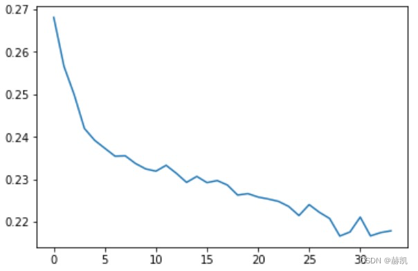
看下损失函数的曲线
plt.plot(history.epoch, history.history['loss'], label='total loss')
plt.show()
生成notes
预测方法
def predict_next_note(
    notes: np.ndarray,
    keras_model: tf.keras.Model,
    temperature: float = 1.0) -> int:
  """Generates a note IDs using a trained sequence model."""

  assert temperature > 0

  # Add batch dimension
  inputs = tf.expand_dims(notes, 0)

  predictions = model.predict(inputs)
  pitch_logits = predictions['pitch']
  step = predictions['step']
  duration = predictions['duration']

  pitch_logits /= temperature
  pitch = tf.random.categorical(pitch_logits, num_samples=1)
  pitch = tf.squeeze(pitch, axis=-1)
  duration = tf.squeeze(duration, axis=-1)
  step = tf.squeeze(step, axis=-1)

  # `step` and `duration` values should be non-negative
  step = tf.maximum(0, step)
  duration = tf.maximum(0, duration)

  return int(pitch), float(step), float(duration)
预测一波
temperature = 2.0
num_predictions = 120

sample_notes = np.stack([raw_notes[key] for key in key_order], axis=1)

# The initial sequence of notes; pitch is normalized similar to training
# sequences
input_notes = (
    sample_notes[:seq_length] / np.array([vocab_size, 1, 1]))

generated_notes = []
prev_start = 0
for _ in range(num_predictions):
  pitch, step, duration = predict_next_note(input_notes, model, temperature)
  start = prev_start + step
  end = start + duration
  input_note = (pitch, step, duration)
  generated_notes.append((*input_note, start, end))
  input_notes = np.delete(input_notes, 0, axis=0)
  input_notes = np.append(input_notes, np.expand_dims(input_note, 0), axis=0)
  prev_start = start

generated_notes = pd.DataFrame(
    generated_notes, columns=(*key_order, 'start', 'end'))
查看预测的数据
generated_notes.head(10)
听一下
out_file = 'output.mid'
out_pm = notes_to_midi(
    generated_notes, out_file=out_file, instrument_name=instrument_name)
display_audio(out_pm)
看一下图
plot_piano_roll(generated_notes)
plot_distributions(generated_notes)
还是蛮有意思的
总结
损失函数的自定义,还有RNN输入数据输出数据的生成
本文来自博客园,作者:赫凯,转载请注明原文链接:https://www.cnblogs.com/heKaiii/p/17137404.html

 浙公网安备 33010602011771号