布匹瑕疵检测数据集EDA分析
分析数据集中 train 集的每个类别的 bboxes 数量分布情况。因为训练集分了两个:train1,train2。先根据两个数据集的 anno_train.json 文件分析类别分布。数据集:布匹瑕疵检测数据集-阿里云天池 (aliyun.com)
| 数据集 | bbox数量 | 缺陷图片数量 | 正常图片数量 |
|---|---|---|---|
| train1 | 7728 | 4774 | 2538 |
| train2 | 1795 | 1139 | 1125 |
| 总共 | 9523 | 5823 | 3663 |
EDA.py
import json
import os
import matplotlib.pyplot as plt
import seaborn as sns
#########################################
# 定义文件路径,修改成自己的anno文件路径
EDA_dir = './EDA/'
if not os.path.exists(EDA_dir):
# shutil.rmtree(EDA_dir)
os.makedirs(EDA_dir)
root_path = os.getcwd()
train1_json_filepath = os.path.join(root_path, "smartdiagnosisofclothflaw_round1train1_datasets",
"guangdong1_round1_train1_20190818", "Annotations",'anno_train.json')
train2_json_filepath = os.path.join(root_path, "smartdiagnosisofclothflaw_round1train2_datasets",
"guangdong1_round1_train2_20190828", "Annotations",'anno_train.json')
#########################################
# 准备数据
data1 = json.load(open(train1_json_filepath, 'r'))
data2 = json.load(open(train2_json_filepath, 'r'))
category_all = []
category_dis = {}
for i in data1:
category_all.append(i["defect_name"])
if i["defect_name"] not in category_dis:
category_dis[i["defect_name"]] = 1
else:
category_dis[i["defect_name"]] += 1
for i in data2:
category_all.append(i["defect_name"])
if i["defect_name"] not in category_dis:
category_dis[i["defect_name"]] = 1
else:
category_dis[i["defect_name"]] += 1
#########################################
# 配置绘图的参数
sns.set_style("whitegrid")
plt.figure(figsize=(15, 9)) # 图片的宽和高,单位为inch
# 绘制第一个子图:类别分布情况
plt.xlabel('class', fontsize=14) # x轴名称
plt.ylabel('counts', fontsize=14) # y轴名称
plt.xticks(rotation=90) # x轴标签竖着显示
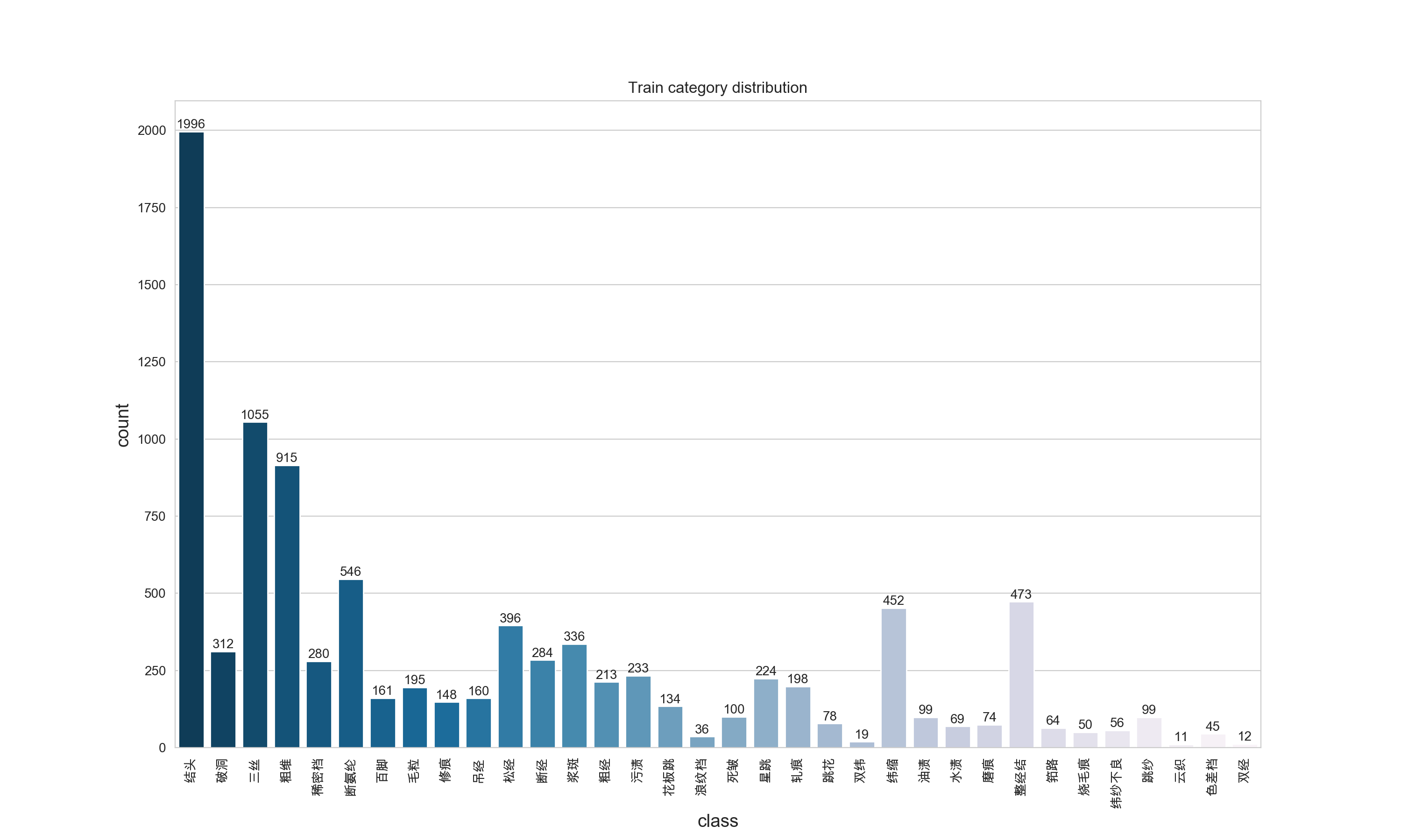
plt.title('Train category distribution') # 标题
category_num = [category_dis[key] for key in category_dis] # 制作一个y轴每个条高度列表
for x, y in enumerate(category_num):
plt.text(x, y + 10, '%s' % y, ha='center', fontsize=10) # x轴偏移量,y轴偏移量,数值,居中,字体大小。
ax = sns.countplot(x=category_all, palette="PuBu_r") # 绘制直方图,palette调色板,蓝色由浅到深渐变。
# palette样式:https://blog.csdn.net/panlb1990/article/details/103851983
plt.savefig(EDA_dir + 'category_distribution.png', dpi=500)
plt.show()
可视化结果展示:
如果你的可视化结果,matplotlib和seaborn不能显示中文,参考这里:解决python中matplotlib与seaborn画图时中文乱码的根本问题 ,亲测有用。
通过可视化结果,我们可以看出数据集中类别极不平衡,最高的1996,最低的11。接下来我们继续分析一下每个类别的宽高分布情况,以及bbox的宽高比分布情况。
EDA.py
import json
import os

import matplotlib.pyplot as plt
import seaborn as sns
#########################################
# 定义文件路径,修改成自己的anno文件路径
EDA_dir = './EDA/'
if not os.path.exists(EDA_dir):
    # shutil.rmtree(EDA_dir)
    os.makedirs(EDA_dir)

root_path = os.getcwd()
train1_json_filepath = os.path.join(root_path, "smartdiagnosisofclothflaw_round1train1_datasets",
                                    "guangdong1_round1_train1_20190818", "Annotations", 'anno_train.json')

train2_json_filepath = os.path.join(root_path, "smartdiagnosisofclothflaw_round1train2_datasets",
                                    "guangdong1_round1_train2_20190828", "Annotations", 'anno_train.json')

#########################################
# 准备数据
data1 = json.load(open(train1_json_filepath, 'r'))
data2 = json.load(open(train2_json_filepath, 'r'))

category_dis = {}
bboxes = {}
widths = {}
heights = {}
aspect_ratio={}

for i in data1:
    if i["defect_name"] not in category_dis:
        category_dis[i["defect_name"]] = 1
        bboxes[i["defect_name"]] = [i["bbox"], ]
    else:
        category_dis[i["defect_name"]] += 1
        bboxes[i["defect_name"]].append(i['bbox'])

for i in data2:
    if i["defect_name"] not in category_dis:
        category_dis[i["defect_name"]] = 1
        bboxes[i["defect_name"]] = [i["bbox"], ]
    else:
        category_dis[i["defect_name"]] += 1
        bboxes[i["defect_name"]].append(i['bbox'])

for i in bboxes:
    widths[i]=[]
    heights[i]=[]
    aspect_ratio[i]=[]
    for j in bboxes[i]:
        x1,y1,x2,y2=j
        widths[i].append(x2-x1)
        heights[i].append(y2-y1)
        aspect_ratio[i].append((x2-x1)/(y2-y1))

#########################################
# 配置绘图的参数
sns.set_style("whitegrid")
plt.figure(figsize=(15, 20))  # 图片的宽和高,单位为inch
plt.subplots_adjust(left=0.1,bottom=0.1,right=0.9,top=0.9,wspace=0.5,hspace=0.5)    # 调整子图间距

# 绘制bbox宽度和高度分布情况
for idx,i in enumerate(bboxes):
    plt.subplot(7,5,idx+1)
    plt.xlabel('width', fontsize=11)  # x轴名称
    plt.ylabel('height', fontsize=11)  # y轴名称
    plt.title(i, fontsize=13)  # 标题
    sns.scatterplot(widths[i],heights[i])

plt.savefig(EDA_dir + 'width_height_distribution.png', dpi=500, pad_inches=0)
plt.show()

# 绘制宽高比分布情况
plt.figure(figsize=(15, 20))  # 图片的宽和高,单位为inch
plt.subplots_adjust(left=0.1,bottom=0.1,right=0.9,top=0.9,wspace=0.5,hspace=0.5)    # 调整子图间距

for idx,i in enumerate(bboxes):
    plt.subplot(7,5,idx+1)
    plt.xlabel('aspect ratio', fontsize=11)  # x轴名称
    plt.ylabel('number', fontsize=11)  # y轴名称
    plt.title(i, fontsize=13)  # 标题
    sns.distplot(aspect_ratio[i],kde=False)

plt.savefig(EDA_dir + 'aspect_ratio_distribution.png', dpi=500, pad_inches=0)
plt.show()
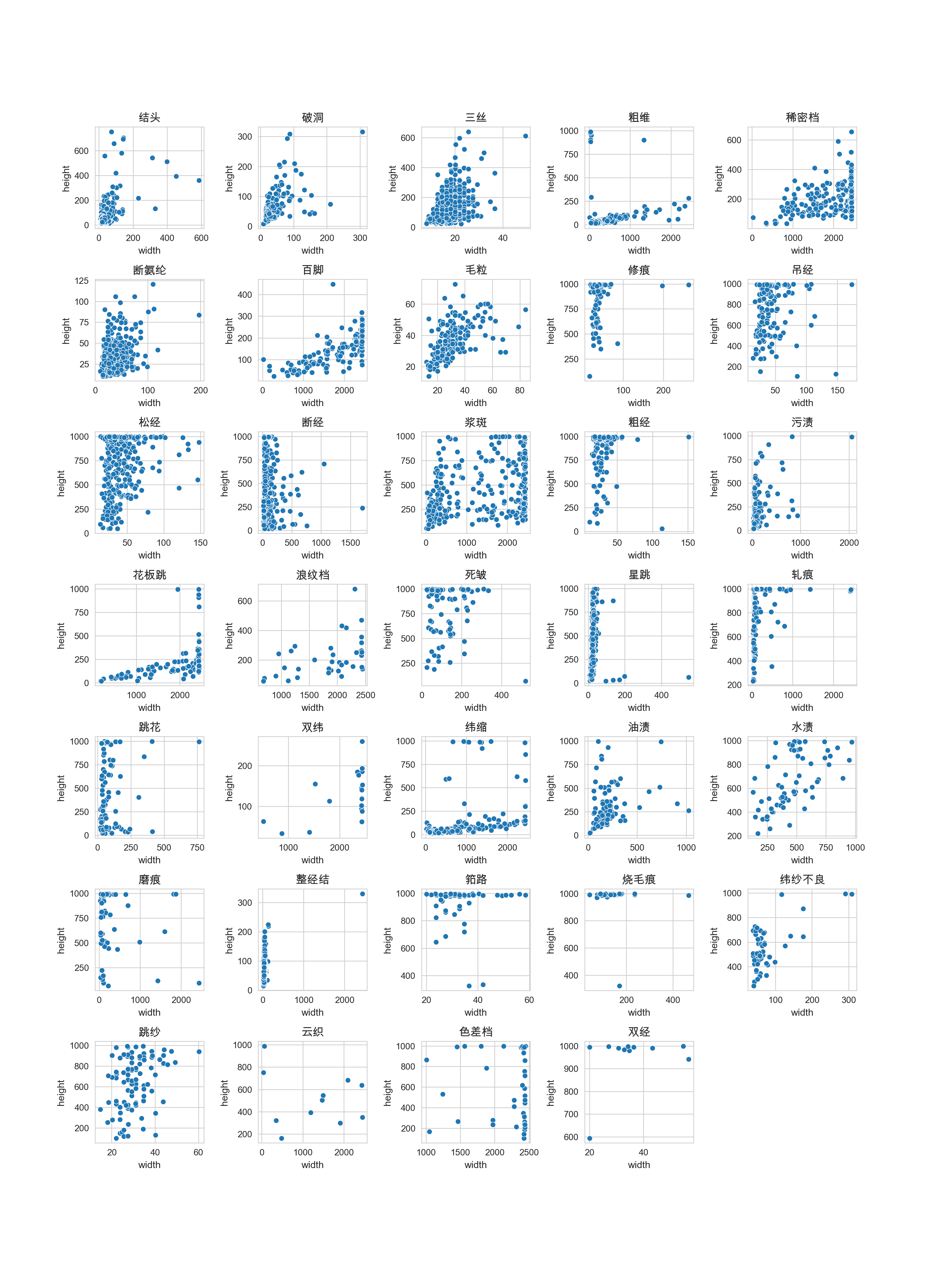
可视化结果展示:bbox宽度和高度分布情况
可视化结果展示:bbox宽高比的分布情况
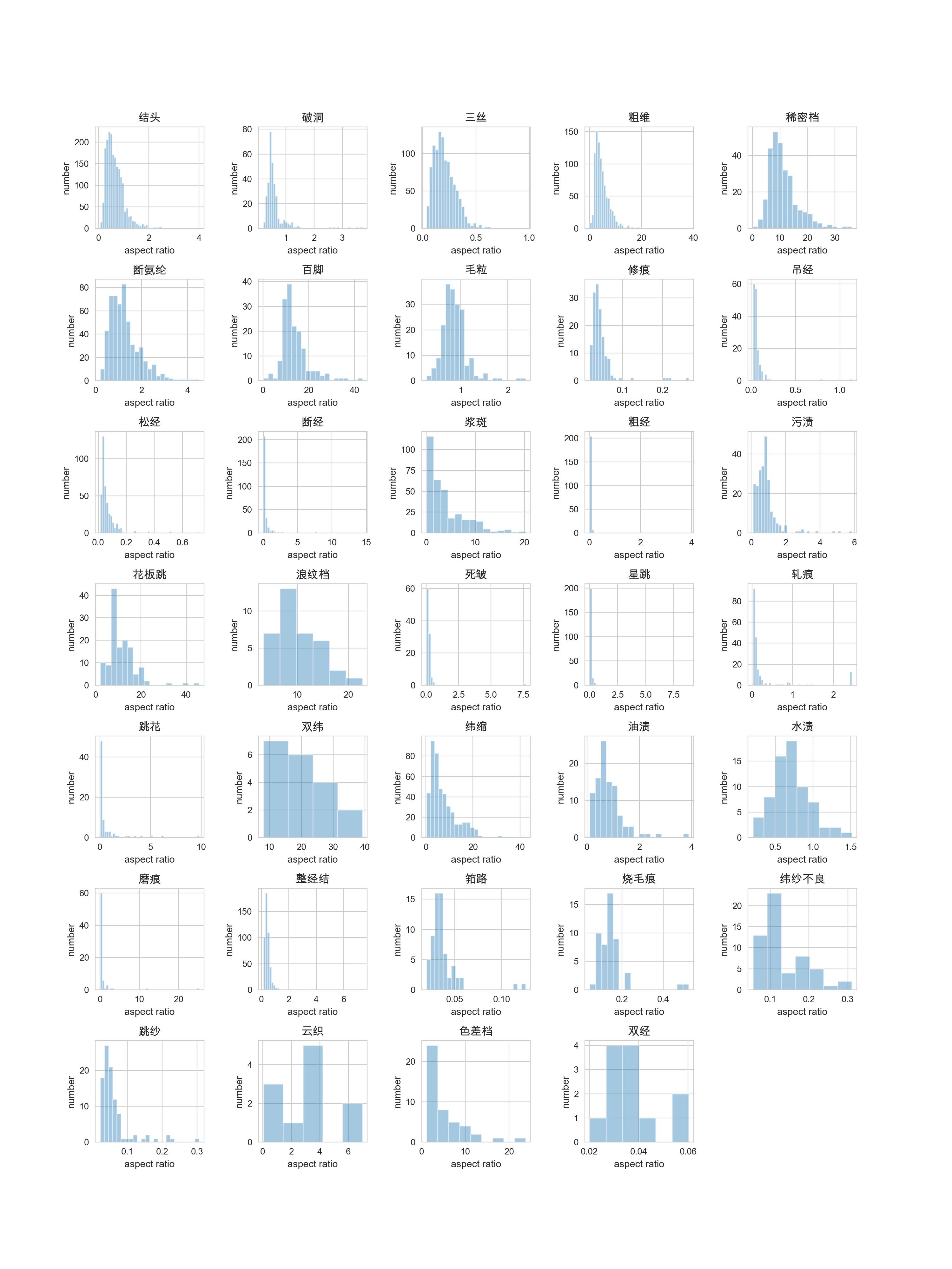
⭐ 做完所有的EDA后,可以得到以下分析:
- bbox的类别分布极不平衡。
- bbox的形状差异很大,粗维,稀密档,百脚等宽高比数值很大,部分大于10,说明bbox呈细条状。需要针对此进行修改,生成特殊比例的anchor。

 浙公网安备 33010602011771号