大作业

一、boston房价预测

1. 读取数据集

2. 训练集与测试集划分

3. 线性回归模型：建立13个变量与房价之间的预测模型，并检测模型好坏。

4. 多项式回归模型：建立13个变量与房价之间的预测模型，并检测模型好坏。

5. 比较线性模型与非线性模型的性能，并说明原因。

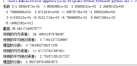
#一、boston房价预测
#导入加载包
from sklearn.datasets import load_boston
from sklearn.model_selection import train_test_split
from sklearn.linear_model import LinearRegression
from sklearn.preprocessing import PolynomialFeatures

# 读取波士顿房价数据集
data = load_boston()

# 划分数据集
x_train, x_test, y_train, y_test = train_test_split(data.data,data.target,test_size=0.2)

# 建立多元线性回归模型
mlr = LinearRegression()
mlr.fit(x_train,y_train)
print('系数',mlr.coef_,"\n截距",mlr.intercept_)

# 检测模型好坏
from sklearn.metrics import regression
y_predict = mlr.predict(x_test)
# 计算模型的预测指标
print("预测的均方误差：", regression.mean_squared_error(y_test,y_predict))
print("预测的平均绝对误差：", regression.mean_absolute_error(y_test,y_predict))
# 打印模型的分数
print("模型的分数：",mlr.score(x_test, y_test))

# 多元多项式回归模型
# 多项式化
poly2 = PolynomialFeatures(degree=2)
x_poly_train = poly2.fit_transform(x_train)
x_poly_test = poly2.transform(x_test)

# 建立模型
mlrp = LinearRegression()
mlrp.fit(x_poly_train, y_train)

# 预测
y_predict2 = mlrp.predict(x_poly_test)
# 检测模型好坏
# 计算模型的预测指标
print("预测的均方误差：", regression.mean_squared_error(y_test,y_predict2))
print("预测的平均绝对误差：", regression.mean_absolute_error(y_test,y_predict2))
# 打印模型的分数
print("模型的分数：",mlrp.score(x_poly_test, y_test))
#线性模型与非线性模型的性能比较：线性模型的图形明显比非线性模型的图像更加贴切形象，平滑的曲线更精确地将样本点的分布规律展现出来，极大地减少了误差，性能更有优势。

二、中文文本分类

1.读取清洗分词

import os
import numpy as np
import sys
from datetime import datetime
import gc
#倒入替换路径
path = r'C:\Users\WZZ\Desktop\147'
#倒入结巴
import jieba
#导入停用词
with open(r'F:\数据挖掘\stopsCN.txt', encoding='utf-8') as f:
    stopwords = f.read().split('\n')
#print(stopwords.shape)#查看停用的字符数量
# for w in stopwords:#查看stopwords文件数据
#     print(w)

#文本预处理
def processing(tokens):
    tokens = "".join([char for char in tokens if char.isalpha()])# 去掉非字母汉字的字符
    tokens = [token for token in jieba.cut(tokens, cut_all=True) if len(token) >= 2]#结巴分词
    tokens = " ".join([token for token in tokens if token not in stopwords])# 去掉停用词
    return tokens

tokenList = []
targetList = []
for root, dirs, files in os.walk(path):
    # print(root)#地址
    # print(dirs)#子目录
    # print(files)#详细文件名
    for f in files:
        filePath = os.path.join(root, f)#地址拼接
        with open(filePath, encoding='utf-8') as f:
            content = f.read()
            #获取类别标签
            target = filePath.split('\\')[-2]
            targetList.append(target)
            tokenList.append(processing(content))
print( tokenList)　

2.预测评估

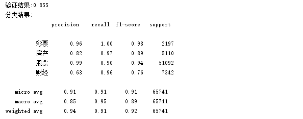
#建模
from sklearn.feature_extraction.text import TfidfVectorizer
from sklearn.model_selection import train_test_split
from sklearn.naive_bayes import GaussianNB, MultinomialNB
from sklearn.model_selection import cross_val_score
from sklearn.metrics import classification_report

x_train, x_test, y_train, y_test = train_test_split(tokenList, targetList, test_size=0.3, stratify=targetList)
#转化特征向量
vectorizer = TfidfVectorizer()
X_train = vectorizer.fit_transform(x_train)
X_test = vectorizer.transform(x_test)
from sklearn.naive_bayes import MultinomialNB
#贝叶斯预测种类
mnb = MultinomialNB()
module = mnb.fit(X_train, y_train)
y_predict = module.predict(X_test)
scores = cross_val_score(mnb, X_test, y_test, cv=5)
print("验证结果:%.3f" % scores.mean())
print("分类结果:\n", classification_report(y_predict, y_test))

3.对比

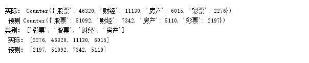
import collections
# 测试集和预测集的各类新闻数量
testCount = collections.Counter(y_test)
predCount = collections.Counter(y_predict)
print('实际：', testCount, '\n', '预测', predCount)
# 建立标签列表，实际结果与预测结果
nameList = list(testCount.keys())
testList = list(testCount.values())
predictList = list(predCount.values())
x = list(range(len(nameList)))
print("类别：", nameList, '\n', "实际：", testList, '\n', "预测：", predictList)

　　

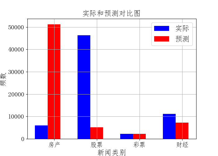
 4.图像对比

# 画图
import matplotlib.pyplot as plt
from pylab import mpl
mpl.rcParams['font.sans-serif'] = ['FangSong'] # 指定字体
plt.figure(figsize=(7,5))
total_width, n = 0.6, 2
width = total_width / n
plt.bar(x, testList, width=width,label='实际',fc = 'blue')
for i in range(len(x)):
    x[i] = x[i] + width
plt.bar(x, predictList,width=width,label='预测',tick_label = nameList,fc='r')
plt.grid()
plt.title('实际和预测对比图',fontsize=17)
plt.xlabel('新闻类别',fontsize=17)
plt.ylabel('频数',fontsize=17)
plt.legend(fontsize =17)
plt.tick_params(labelsize=15)
plt.show()