使用OPTUNA对LightBGM自动调试参数，并进行绘图可视化

 

1.optuna基本使用 

Optuna是一个自动帮助我们调试参数的工具，使用起来十分方便。比sklearn的gridsearchcv好用很多，一是因为optuna相比于sklearn能够快速进行调参，二是因为它可以将调试参数的过程进行可视化。同时可以如果没训练完，下次继续训练。而optuna内部使用贝叶斯调试参数的机制，可以在最短的时间之内，给我们一个较为优秀的结果，甚至可能会得到一个最优的结果。我们可以根据贝叶斯调参给我们确定的参数范围，自行使用gird search再次验证最佳参数，当然这在大部分情况下没必要了。

我们首先先在函数里使用k折交叉验证，这里使用5折交叉验证，对我们的结果进行优化，当然你也可以使用10折交叉验证。

在函数train_model_category当中，我们一共有三个参数，trail，data，y。trail是optuna自带的一个传入参数，我们在调用train_model_category会使用到它。data是我们训练集的数据，y是训练集的label。函数return的变量则是当前k折交叉验证得到的一个auc（accuracy）的值，因此你可以在这里完全自定义你用来评价的指标，可以是auc，mse，也可以是accuracy均可。optuna完全是一个开放的框架。

在我们的字典 param_grid当中，传入了lightbgm常用的参数，

其中，例如：

"n_estimators": trial.suggest_int("n_estimators", 5000,10000,step=1000),

这里使用调试了n_estimator的参数，suggest_int表示我们在后面的参数是int型变量。因为有些参数可能是小数，也就是浮点型的数据，这个时候我们就需要考虑使用suggest_float 了。step表示，参数可以从5000-10000之间波动，每一次波动的step为1000.因此我们的n_estimator的参数可能的范围是（5000，6000，7000，8000，9000，10000）.

import optuna
from optuna.integration import LightGBMPruningCallback

from sklearn.model_selection import KFold

 def train_model_category(trial,data_,y_):
   #使用sklearn建立fold
    folds_ = KFold(n_splits=5, shuffle=True, random_state=546789)
    param_grid = {
        "n_estimators": trial.suggest_int("n_estimators", 5000,10000,step=1000),
        "learning_rate": trial.suggest_float("learning_rate", 0.01, 0.3,step=0.05),
        "num_leaves": trial.suggest_int("num_leaves", 2**2, 2**5, step=4),
        "max_depth": trial.suggest_int("max_depth", 3, 12,step=2),
        "min_data_in_leaf": trial.suggest_int("min_data_in_leaf", 200, 10000, step=100),
        "lambda_l1": trial.suggest_int("lambda_l1", 0, 100, step=5),
        "lambda_l2": trial.suggest_int("lambda_l2", 0, 100, step=5),
        "min_gain_to_split": trial.suggest_float("min_gain_to_split", 0, 15),
        "bagging_fraction": trial.suggest_float("bagging_fraction", 0.2, 0.95, step=0.1),
        "bagging_freq": trial.suggest_categorical("bagging_freq", [1]),
        "feature_fraction": trial.suggest_float("feature_fraction", 0.2, 0.95, step=0.1),
        "colsample_bytree":trial.suggest_float("colsample_bytree", 0.2, 0.9, step=0.1),
        "subsample":trial.suggest_float("subsample", 0.2, 1, step=0.1),
        "reg_alpha":trial.suggest_float("reg_alpha", 0.2, 1, step=0.1),
        "random_state": 2021,
    }
    oof_preds = np.zeros(data_.shape[0])
    sub_preds = np.zeros(test_.shape[0])
    feature_importance_df = pd.DataFrame()
　　#这里去除无关的特征，load id，user id，is default
    feats = [f for f in data_.columns if f not in ['loan_id', 'user_id', 'isDefault'] ]
    for n_fold, (trn_idx, val_idx) in enumerate(folds_.split(data_)):
        trn_x, trn_y = data_[feats].iloc[trn_idx], y_.iloc[trn_idx]
        val_x, val_y = data_[feats].iloc[val_idx], y_.iloc[val_idx]
        clf = LGBMClassifier(**param_grid)
        
        clf.fit(trn_x, trn_y, 
                eval_set= [(trn_x, trn_y), (val_x, val_y)], 
                eval_metric='auc', verbose=100,
                early_stopping_rounds=40  #30
               )

        oof_preds[val_idx] = clf.predict_proba(val_x, num_iteration=clf.best_iteration_)[:, 1]

　　　　 del clf, trn_x, trn_y, val_x, val_y
        gc.collect()
        
    print('Full AUC score %.6f' % roc_auc_score(y, oof_preds)) 
    
    return roc_auc_score(y, oof_preds)

然后定义优化函数：

study = optuna.create_study(direction="maximize", study_name="LGBM Classifier")
func = lambda trial: train_model_category(trial,train, y)
study.optimize(func, n_trials=20)

这里传入的参数trial，train和y。同时自定义direction=“maximize”，如果是mse，则可以定义为“minimize”。

现在运行代码，就可以调试参数啦！

2.optuna超参数空间可视化

首先导入相关的包：

from optuna.visualization import plot_contour
from optuna.visualization import plot_edf
from optuna.visualization import plot_intermediate_values
from optuna.visualization import plot_optimization_history
from optuna.visualization import plot_parallel_coordinate
from optuna.visualization import plot_param_importances
from optuna.visualization import plot_slice

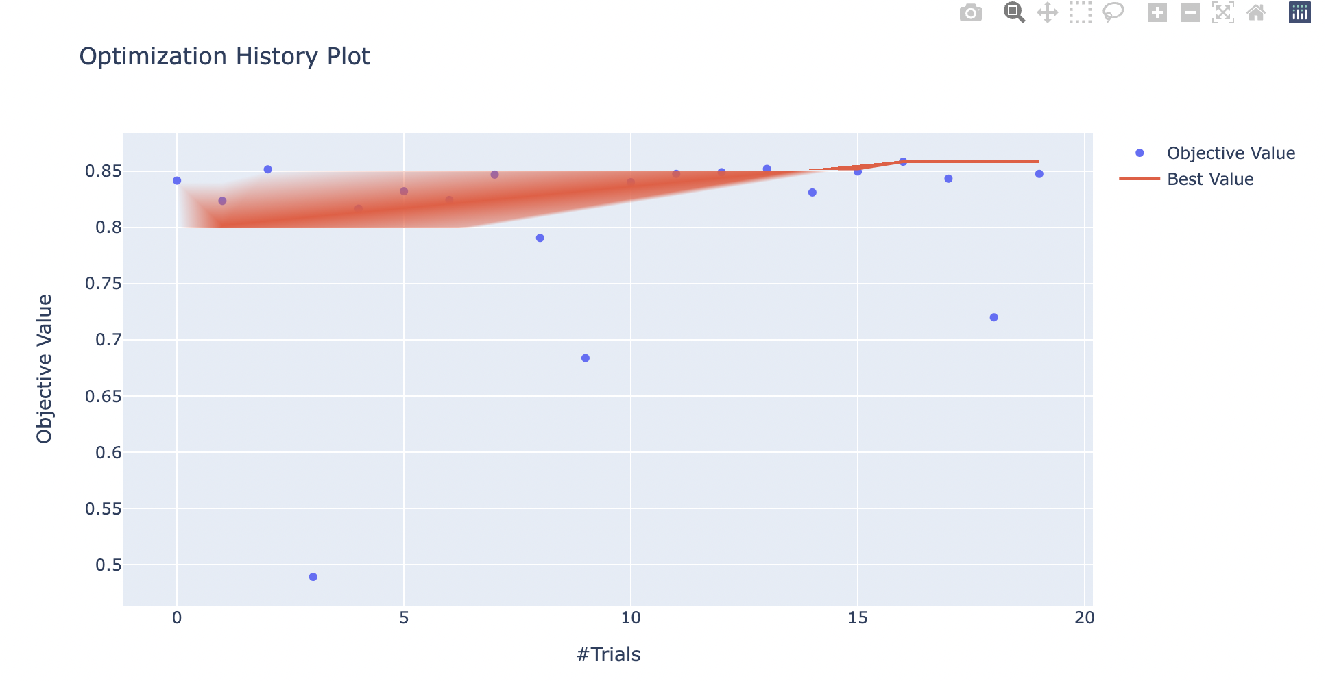
绘制参数优化的历史图像：

plot_optimization_history(study)

 

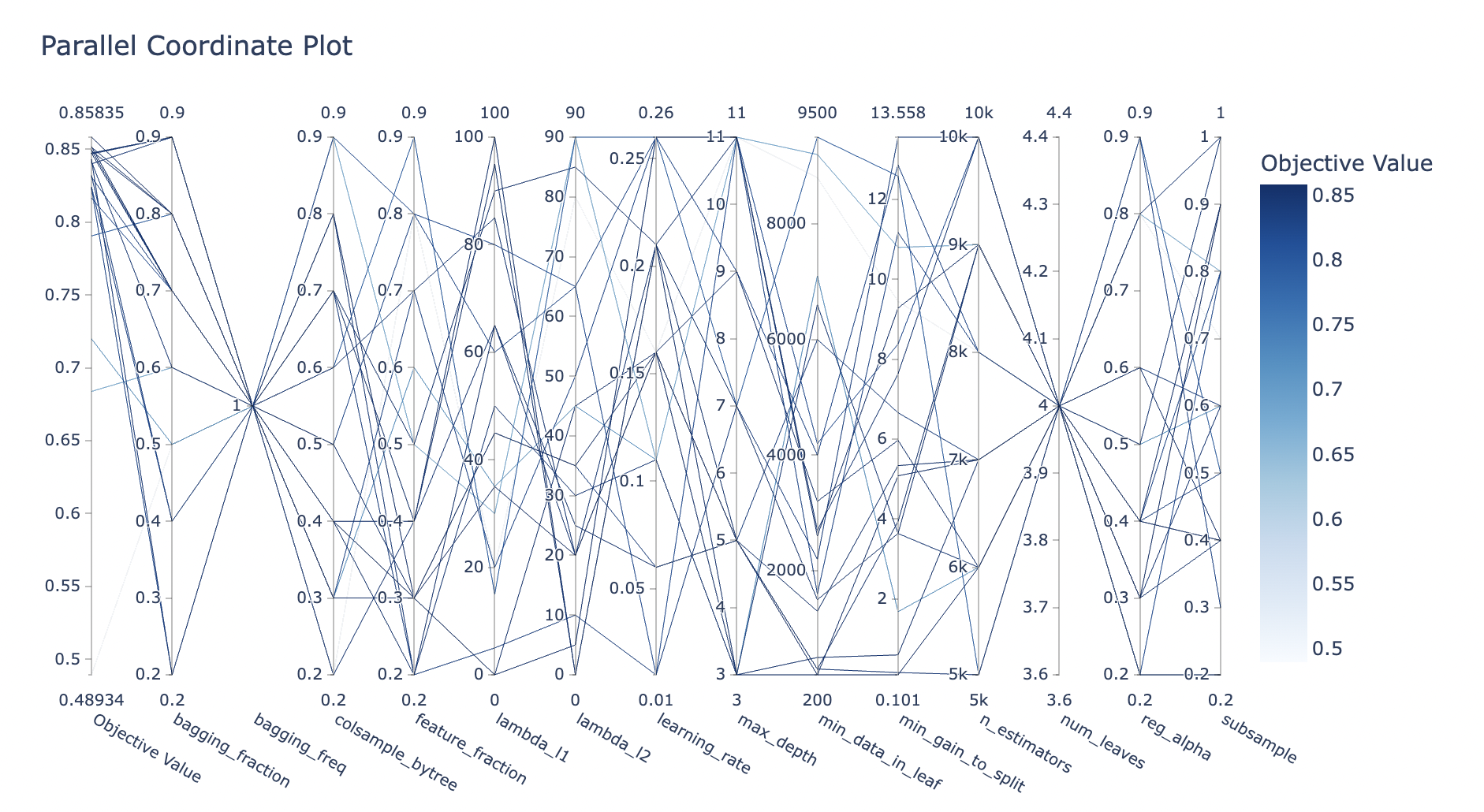
 绘制参数之间高纬度关系：

#绘制高纬关系
plot_parallel_coordinate(study)

 

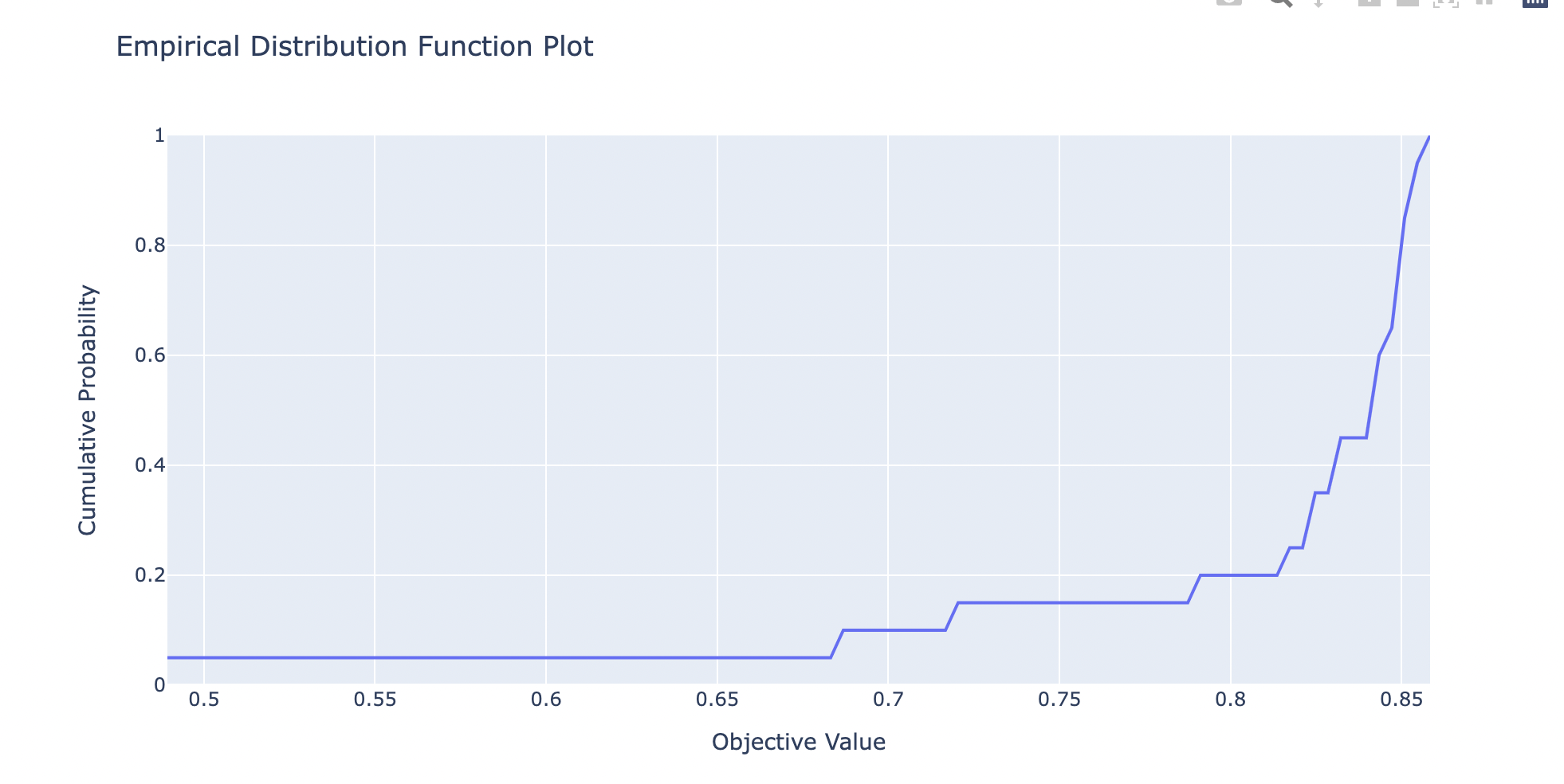
 绘制经验分布函数：

#绘制经验分布函数
plot_edf(study)

 

 这就是今天的optuna绘制教程啦！觉得有收获的别忘记点下方的赞和推荐呀！