torch.nn中的网络模型介绍

一、torch.nn.Linear

torch.nn.Linear（in_features,out_features,bias=True）

nn.linear()是用来设置网络中的全连接层的，也可以说是线性映射，这里面没有激活函数。而在全连接层中的输入与输出都是二维张量，输入输出的形状为[batch_size, size]

import torch
from IPython.core.interactiveshell import  InteractiveShell
InteractiveShell.ast_node_interactivity='all'

#输入=【128，20】，128个样本，维度20
x = torch.randn(128, 20) 
#通过全连接做线性变换，从20维转化为30维度
m = torch.nn.Linear(20, 30)  # 20,30是指维度
#输出的size=【128，30】，128个样本，每个样本维度30
output = m(x)


output.shape
m.weight.shape
m.bias.shape

torch.Size([128, 30])

torch.Size([30, 20])

torch.Size([30])

二、torch.nn.LSTM

input_size ：输入的维度
hidden_size：h的维度
num_layers：堆叠LSTM的层数，默认值为1,这里的层数表示是单层还是双层的
bias：偏置 ，默认值：True
batch_first： 如果是True，则input为(batch, seq, input_size)。默认值为：False（seq_len, batch, input_size）
bidirectional ：是否双向传播，默认值为False

以训练句子为例子，假如每个词是100维的向量，每个句子含有24个单词，一次训练10个句子。那么batch_size=10,seq=24,input_size=100。(seq指的是句子的长度，input_size作为一个的输入) ，所以在设置LSTM网络的过程中input_size=100。由于seq的长度是24，那么这个LSTM结构会循环24次最后输出预设的结果，所以如果是单层的lstm，其实就是一个lstm循环seq次，如果是num_layers=2，就是上下两层lstm循环seq次。

 

(num_layers,bidirectional)，两个的结构的区别如下图所示：

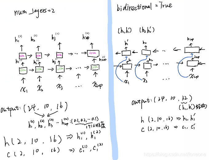
输出：
output ：（seq_len,batch_size, num_directions * hidden_size）
h_n：(num_layers * num_directions, batch, hidden_size)
c_n ：（num_layers * num_directions, batch, hidden_size）

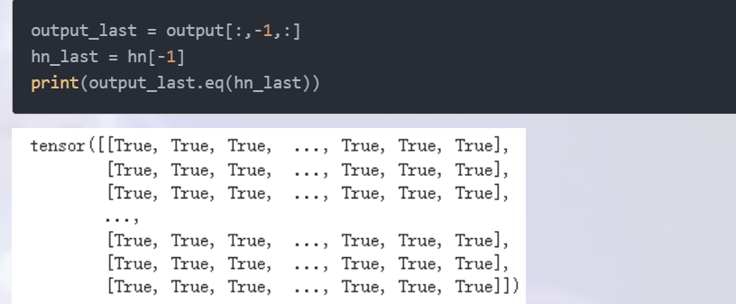
output：保存了每个时间步的输出，如果想要获取最后一个时间步的输出，则可以这么获取：output_last = output[:,-1,:]
h_n：包含的是句子的最后一个单词的隐藏状态，与句子的长度seq_length无关
c_n：包含的是句子的最后一个单词的细胞状态，与句子的长度seq_length无关

另外：最后一个时间步的输出等于最后一个隐含层的输出:

 

import torch.nn as nn
import torch
#seq=24，batch=10，input_size=100
x = torch.rand(24,10,100)
#input_size=100,hide_size=16
lstm = nn.LSTM(100,16,num_layers=2)
#结果输出
output,(h,c) = lstm(x)
print(output.size())
print(h.size())
print(c.size())

 
output:
#这个表示的是最终10个长度为24的句子的最终的输出
torch.Size([24, 10, 16])
#因为是上下两层的lstm，所以有两组h和c
torch.Size([2, 10, 16])
torch.Size([2, 10, 16])

 如果设置为batch_first=True，就代表输入中第一个是batch_size,最后输出也会变化了，如下：

import torch.nn as nn
import torch
#batch=10，seq=24，input_size=100
x = torch.rand(24,10,100)
#input_size=100,hide_size=16
lstm = nn.LSTM(100,16,num_layers=2,batch_first=True)
#结果输出
output,(h,c) = lstm(x)
print(output.size())
print(h.size())
print(c.size())

OUT:
torch.Size([24, 10, 16])
torch.Size([2, 24, 16])
torch.Size([2, 24, 16])

 可以根据seq的长度一个一个步长的循环输入：

import torch
import torch.nn as nn
lstm = nn.LSTM(10, 20, 2)
x = torch.randn(5, 3, 10)
h0 = torch.randn(2, 3, 20)
c0 = torch.randn(2, 3, 20)
hn,cn=h0,c0
#可以根据seq的长度一个一个循环输入
for i in range(len(x)):
    #x[i]后就少了一个维度了，所以需要前面再加入一个维度unsqueeze(0)
    output, (hn, cn)=lstm(x[i].unsqueeze(0), (hn, cn))
    print(output.shape)#这个时候output的输出就不是整体所有步长的了，而是一个一个步长的输出了。

OUT:

torch.Size([1, 3, 20]) 
torch.Size([1, 3, 20])
torch.Size([1, 3, 20])
torch.Size([1, 3, 20])
torch.Size([1, 3, 20])

 三、torch.nn.Conv1d

class torch.nn.Conv1d(in_channels, out_channels, kernel_size,stride=1, padding=0, dilation=1, groups=1, bias=True)
in_channels(int)—输入数据的通道数。在文本分类中，即为句子中单个词的词向量的维度。 （word_vector_num）
out_channels(int)—输出数据的通道数。设置 N 个输出通道数，就有 N 个1维卷积核。（new word_vector_num）
kernel_size(int or tuple) —卷积核的长度，1维卷积中卷积核的实际大小维度是（in_channels，kernel_size），顺序不可互换。
stride(int or tuple, optional)—卷积步长,步长就是一次卷积核移动多元，可以移动2步，也可以一步步移动。
padding (int or tuple, optional)—输入的每一条边补充0的层数。
dilation(int or tuple, `optional``)—卷积核元素之间的间距。
groups(int, optional)—从输入通道到输出通道的阻塞连接数。
bias(bool, optional)—如果bias=True，添加偏置。
举例：

import torch as t
input = t.randn(6,5,3) # batch_size= 6(sentence_num), sentence_word_num= 5, word_vector_num = 3
print(input)
print(input.shape) # [6,5,3]
input = input.permute(0,2,1) # 维度转换(sentence_word_num <-> word_vector_num) 
print(input)
print(input.shape) # [6,3,5]
conv1 = nn.Conv1d(3, 8, 2, bias=False) # in_channels = word_vector_num = 3,out_channels = 8(new word_vector_num), kernel_size = 2
print(conv1.weight.shape) # [8,3,2]
output = conv1(input)
print(output)
print(output.shape) # [6,8,4]

详细参考：https://blog.csdn.net/rothschild666/article/details/124127319

Conv1d&kernel_size=1和nn.linear()有什么不同呢？

import torch
import torch.nn as nn
import torch.nn.functional as F

x = torch.randn(1, 100, 3)        # 创建一个batch_size=1的点云，长度100
layer = nn.Linear(3, 10)        # 构造一个输入节点为3，输出节点为10的网络层
y = F.sigmoid(layer(x))            # 计算y，sigmoid激活函数

print(x.size())
print(y.size())
'''
>>>torch.Size([1, 100, 3])
>>>torch.Size([1, 100, 10])

换成Conv1d来看看：

import torch
import torch.nn as nn
import torch.nn.functional as F
#先进行了转置
x = torch.randn(1, 3, 100)                    # 创建一个batch_size=1的点云，长度100
layer = nn.Conv1d(3, 10, kernel_size=1)        # 构造一个输入节点为3，输出节点为10的网络层
y = F.sigmoid(layer(x))                         # 计算y，sigmoid激活函数

print(x.size())
print(y.size())
'''
>>>torch.Size([1, 3, 100])
>>>torch.Size([1, 10, 100])#若要结果与线性变换一直，可以最后对结果再转置回来。

 

1、nn.Conv1d输入的是一个[batch, channel, length]，3维tensor，而nn.Linear输入的是一个[batch, *, in_features]，可变形状tensor，在进行等价计算时务必保证nn.Linear输入tensor为三维
2、nn.Conv1d作用在第二个维度位置channel，nn.Linear作用在第三个维度位置in_features，对于一个 X X X，若要在两者之间进行等价计算，需要进行tensor.permute，重新排列维度轴秩序，这种情况下如果参数也是一致的，其计算结果就是一样的。

验证nn.Conv1d, kernel_size=1与nn.Linear计算结果相同

 

import torch

def count_parameters(model):
    """Count the number of parameters in a model."""
    return sum([p.numel() for p in model.parameters()])

conv = torch.nn.Conv1d(8,32,1)
print(count_parameters(conv))
# 288

linear = torch.nn.Linear(8,32)
print(count_parameters(linear))
# 288

print(conv.weight.shape)
# torch.Size([32, 8, 1])
print(linear.weight.shape)
# torch.Size([32, 8])

# use same initialization
linear.weight = torch.nn.Parameter(conv.weight.squeeze(2))
linear.bias = torch.nn.Parameter(conv.bias)

tensor = torch.randn(128,256,8)
permuted_tensor = tensor.permute(0,2,1).clone().contiguous()    # 注意此处进行了维度重新排列

out_linear = linear(tensor)
print(out_linear.mean())
# tensor(0.0067, grad_fn=<MeanBackward0>)

out_conv = conv(permuted_tensor)
print(out_conv.mean())
# tensor(0.0067, grad_fn=<MeanBackward0>)