Data Manipulation with dplyr in R
目录
Data Manipulation with dplyr in R
select
select(data,变量名)
The filter and arrange verbs
arrange
counties_selected <- counties %>%
  select(state, county, population, private_work, public_work, self_employed)

# Add a verb to sort in descending order of public_work
counties_selected %>%arrange(desc(public_work))
filter
counties_selected <- counties %>%
  select(state, county, population)

# Filter for counties in the state of California that have a population above 1000000
counties_selected %>%
  filter(state == "California",
         population > 1000000)
#筛选多个变量
filter(id %in% c("a","b","c"...)) 存在
filter(id %in% c("a","b","c"...)) 不存在
fct_relevel
Reorder factor levels by hand
排序,order不好使的时候
f <- factor(c("a", "b", "c", "d"), levels = c("b", "c", "d", "a"))
fct_relevel(f)
fct_relevel(f, "a")
fct_relevel(f, "b", "a")

# Move to the third position
fct_relevel(f, "a", after = 2)

# Relevel to the end
fct_relevel(f, "a", after = Inf)
fct_relevel(f, "a", after = 3)

# Revel with a function
fct_relevel(f, sort)
fct_relevel(f, sample)
fct_relevel(f, rev)
Filtering and arranging
 counties_selected <- counties %>%
    select(state, county, population, private_work, public_work, self_employed)
>
> # Filter for Texas and more than 10000 people; sort in descending order of private_work
> counties_selected %>%filter(state=='Texas',population>10000)%>%arrange(desc(private_work))
# A tibble: 169 x 6
   state county  population private_work public_work self_employed
   <chr> <chr>        <dbl>        <dbl>       <dbl>         <dbl>
 1 Texas Gregg       123178         84.7         9.8           5.4
 2 Texas Collin      862215         84.1        10             5.8
 3 Texas Dallas     2485003         83.9         9.5           6.4
 4 Texas Harris     4356362         83.4        10.1           6.3
 5 Texas Andrews      16775         83.1         9.6           6.8
 6 Texas Tarrant    1914526         83.1        11.4           5.4
 7 Texas Titus        32553         82.5        10             7.4
 8 Texas Denton      731851         82.2        11.9           5.7
 9 Texas Ector       149557         82          11.2           6.7
10 Texas Moore        22281         82          11.7           5.9
# ... with 159 more rows
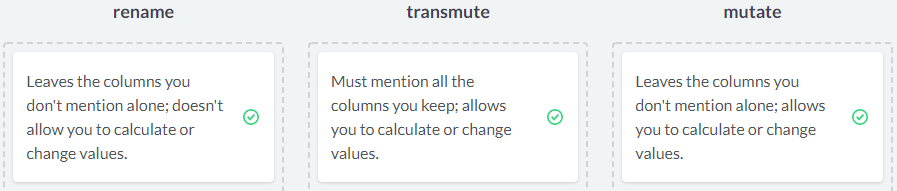
Mutate
counties_selected <- counties %>%
  select(state, county, population, public_work)

# Sort in descending order of the public_workers column
counties_selected %>%
  mutate(public_workers = public_work * population / 100) %>%arrange(desc(public_workers))
counties %>%
  # Select the five columns
  select(state, county, population, men, women) %>%
  # Add the proportion_men variable
  mutate(proportion_men = men / population) %>%
  # Filter for population of at least 10,000
  filter(population >= 10000) %>%
  # Arrange proportion of men in descending order
  arrange(desc(proportion_men))
The count verb
counties_selected %>%count(region,sort=TRUE)
counties_selected %>%count(state,wt=citizens,sort=TRUE)
Summarizing
# Summarize to find minimum population, maximum unemployment, and average income
counties_selected %>%summarize(
min_population=min(population),
max_unemployment=max(unemployment),
average_income=mean(income)
)
# Add a density column, then sort in descending order
counties_selected %>%
  group_by(state) %>%
  summarize(total_area = sum(land_area),
            total_population = sum(population),
            density=total_population/total_area) %>%arrange(desc(density))
发现了,归根到底是一种函数关系,看看该怎样处理这个函数比较简单,如果写不出来,可能和小学的时候应用题写不出来有关系
top_n
按照优先级来筛选
# Extract the most populated row for each state
counties_selected %>%
  group_by(state, metro) %>%
  summarize(total_pop = sum(population)) %>%
  top_n(1, total_pop)
Selecting
Using the select verb, we can answer interesting questions about our dataset by focusing in on related groups of verbs.
The colon (😃 is useful for getting many columns at a time.
In the video you learned about the select helper starts_with(). Another select helper is ends_with(), which finds the columns that end with a particular string.
counties %>%
  # Select the state, county, population, and those ending with "work"
  select(state, county, population, ends_with("work")) %>%
  # Filter for counties that have at least 50% of people engaged in public work
  filter(public_work >= 50)
我觉得这种简单的逻辑关系不应该出错,但是老是出错。。是我真的不太适合做编程这一行嘛?
rename
rename()进行重命名
# Rename the n column to num_counties
counties %>%
  count(state)%>%rename(num_counties=n)
也可以在select的时候直接重命名
 # Select state, county, and poverty as poverty_rate
> counties %>%select(state,county,poverty_rate=poverty)
# A tibble: 3,138 x 3
   state   county   poverty_rate
   <chr>   <chr>           <dbl>
 1 Alabama Autauga          12.9
 2 Alabama Baldwin          13.4
 3 Alabama Barbour          26.7
 4 Alabama Bibb             16.8
 5 Alabama Blount           16.7
 6 Alabama Bullock          24.6
 7 Alabama Butler           25.4
 8 Alabama Calhoun          20.5
 9 Alabama Chambers         21.6
10 Alabama Cherokee         19.2
# ... with 3,128 more rows
transmute
combination select & mutate
类似于mutate,添加新列但是只保留新列,删掉旧列
官方解释: use to calculate new columns while dropping other columns
counties %>%
  # Keep the state, county, and populations columns, and add a density column
  transmute(state, county, population, density = population / land_area) %>%
  # Filter for counties with a population greater than one million
  filter(population > 1000000) %>%
  # Sort density in ascending order
  arrange(density
这个解释挺好的
给出一个综合的例子
> # Change the name of the unemployment column
> counties %>%
    rename(unemployment_rate = unemployment)
# A tibble: 3,138 x 40
   census_id state county region metro population   men women hispanic white
   <chr>     <chr> <chr>  <chr>  <chr>      <dbl> <dbl> <dbl>    <dbl> <dbl>
 1 1001      Alab~ Autau~ South  Metro      55221 26745 28476      2.6  75.8
 2 1003      Alab~ Baldw~ South  Metro     195121 95314 99807      4.5  83.1
 3 1005      Alab~ Barbo~ South  Nonm~      26932 14497 12435      4.6  46.2
 4 1007      Alab~ Bibb   South  Metro      22604 12073 10531      2.2  74.5
 5 1009      Alab~ Blount South  Metro      57710 28512 29198      8.6  87.9
 6 1011      Alab~ Bullo~ South  Nonm~      10678  5660  5018      4.4  22.2
 7 1013      Alab~ Butler South  Nonm~      20354  9502 10852      1.2  53.3
 8 1015      Alab~ Calho~ South  Metro     116648 56274 60374      3.5  73
 9 1017      Alab~ Chamb~ South  Nonm~      34079 16258 17821      0.4  57.3
10 1019      Alab~ Chero~ South  Nonm~      26008 12975 13033      1.5  91.7
# ... with 3,128 more rows, and 30 more variables: black <dbl>, native <dbl>,
#   asian <dbl>, pacific <dbl>, citizens <dbl>, income <dbl>, income_err <dbl>,
#   income_per_cap <dbl>, income_per_cap_err <dbl>, poverty <dbl>,
#   child_poverty <dbl>, professional <dbl>, service <dbl>, office <dbl>,
#   construction <dbl>, production <dbl>, drive <dbl>, carpool <dbl>,
#   transit <dbl>, walk <dbl>, other_transp <dbl>, work_at_home <dbl>,
#   mean_commute <dbl>, employed <dbl>, private_work <dbl>, public_work <dbl>,
#   self_employed <dbl>, family_work <dbl>, unemployment_rate <dbl>,
#   land_area <dbl>
>
> # Keep the state and county columns, and the columns containing poverty
> counties %>%
    select(state, county, contains("poverty"))
# A tibble: 3,138 x 4
   state   county   poverty child_poverty
   <chr>   <chr>      <dbl>         <dbl>
 1 Alabama Autauga     12.9          18.6
 2 Alabama Baldwin     13.4          19.2
 3 Alabama Barbour     26.7          45.3
 4 Alabama Bibb        16.8          27.9
 5 Alabama Blount      16.7          27.2
 6 Alabama Bullock     24.6          38.4
 7 Alabama Butler      25.4          39.2
 8 Alabama Calhoun     20.5          31.6
 9 Alabama Chambers    21.6          37.2
10 Alabama Cherokee    19.2          30.1
# ... with 3,128 more rows
>
> # Calculate the fraction_women column without dropping the other columns
> counties %>%
    mutate(fraction_women = women / population)
# A tibble: 3,138 x 41
   census_id state county region metro population   men women hispanic white
   <chr>     <chr> <chr>  <chr>  <chr>      <dbl> <dbl> <dbl>    <dbl> <dbl>
 1 1001      Alab~ Autau~ South  Metro      55221 26745 28476      2.6  75.8
 2 1003      Alab~ Baldw~ South  Metro     195121 95314 99807      4.5  83.1
 3 1005      Alab~ Barbo~ South  Nonm~      26932 14497 12435      4.6  46.2
 4 1007      Alab~ Bibb   South  Metro      22604 12073 10531      2.2  74.5
 5 1009      Alab~ Blount South  Metro      57710 28512 29198      8.6  87.9
 6 1011      Alab~ Bullo~ South  Nonm~      10678  5660  5018      4.4  22.2
 7 1013      Alab~ Butler South  Nonm~      20354  9502 10852      1.2  53.3
 8 1015      Alab~ Calho~ South  Metro     116648 56274 60374      3.5  73
 9 1017      Alab~ Chamb~ South  Nonm~      34079 16258 17821      0.4  57.3
10 1019      Alab~ Chero~ South  Nonm~      26008 12975 13033      1.5  91.7
# ... with 3,128 more rows, and 31 more variables: black <dbl>, native <dbl>,
#   asian <dbl>, pacific <dbl>, citizens <dbl>, income <dbl>, income_err <dbl>,
#   income_per_cap <dbl>, income_per_cap_err <dbl>, poverty <dbl>,
#   child_poverty <dbl>, professional <dbl>, service <dbl>, office <dbl>,
#   construction <dbl>, production <dbl>, drive <dbl>, carpool <dbl>,
#   transit <dbl>, walk <dbl>, other_transp <dbl>, work_at_home <dbl>,
#   mean_commute <dbl>, employed <dbl>, private_work <dbl>, public_work <dbl>,
#   self_employed <dbl>, family_work <dbl>, unemployment <dbl>,
#   land_area <dbl>, fraction_women <dbl>
>
> # Keep only the state, county, and employment_rate columns
> counties %>%
    transmute(state, county, employment_rate = employed / population)
# A tibble: 3,138 x 3
   state   county   employment_rate
   <chr>   <chr>              <dbl>
 1 Alabama Autauga            0.434
 2 Alabama Baldwin            0.441
 3 Alabama Barbour            0.319
 4 Alabama Bibb               0.367
 5 Alabama Blount             0.384
 6 Alabama Bullock            0.362
 7 Alabama Butler             0.384
 8 Alabama Calhoun            0.406
 9 Alabama Chambers           0.402
10 Alabama Cherokee           0.390
# ... with 3,128 more rows
貌似忘记%in%符号的使用了,复习一下啊
# Filter for the names Steven, Thomas, and Matthew
selected_names <- babynames %>%
  filter(name %in% c("Steven", "Thomas", "Matthew"))
Grouped mutates
这个就是两两组合之前的例子中有的

 浙公网安备 33010602011771号