论文解析 -- How Good Are Query Optimizers, Really? (TUM PVLDB 2015)
INTRODUCTION
The problem of finding a good join order is one of the most studied problems in the database field.
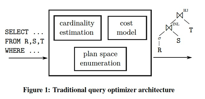
Figure 1 illustrates the classical, cost-based approach, which dates back to System R [36].
这里开宗明义,本文探讨优化器中核心的3个模块,如图,其实优化器所有的研究基本都是这3个方面
所以需要回答的3个问题是,基数估计能做到多准,并对于查询计划的选择的影响多大;代价模型有多重要;空间enumerate需要做多大
To obtain an efficient query plan, the query optimizer enumerates some subset of the valid join orders, for example using dynamic programming.
Using cardinality estimates as its principal input, the cost model then chooses the cheapest alternative from semantically equivalent plan alternatives.
Theoretically, as long as the cardinality estimations and the cost model are accurate, this architecture obtains the optimal query plan.
In reality, cardinality estimates are usually computed based on simplifying assumptions like uniformity and independence.
In realworld data sets, these assumptions are frequently wrong, which may lead to sub-optimal and sometimes disastrous plans.
In this experiments and analyses paper we investigate the three main components of the classical query optimization architecture in order to answer the following questions:
- How good are cardinality estimators and when do bad estimates lead to slow queries?
- How important is an accurate cost model for the overall query optimization process?
- How large does the enumerated plan space need to be?
To answer these questions, we use a novel methodology that allows us to isolate the influence of the individual optimizer components on query performance.
Our experiments are conducted using a realworld data set and 113 multi-join queries that provide a challenging, diverse, and realistic workload.
Another novel aspect of this paper is that it focuses on the increasingly common main-memory scenario, where all data fits into RAM.
The main contributions of this paper are listed in the following:
- We design a challenging workload named Join Order Benchmark (JOB), which is based on the IMDB data set.
The benchmark is publicly available to facilitate further research.
- To the best of our knowledge, this paper presents the first end-to-end study of the join ordering problem using a realworld data set and realistic queries.
- By quantifying the contributions of cardinality estimation, the cost model, and the plan enumeration algorithm on query performance,
we provide guidelines for the complete design of a query optimizer. We also show that many disastrous plans can easily be avoided.
BACKGROUND AND METHODOLOGY
之前的研究大体分为只关注search space或是只考虑基数估计,这些方法都没有考虑实际的场景,比较难落地。
Many query optimization papers ignore cardinality estimation and only study search space exploration for join ordering with randomly generated, synthetic queries (e.g., [32, 13]).
Other papers investigate only cardinality estimation in isolation either theoretically (e.g., [21]) or empirically (e.g., [43]).
As important and interesting both approaches are for understanding query optimizers, they do not necessarily reflect real-world user experience.
The goal of this paper is to investigate the contribution of all relevant query optimizer components to end-to-end query performance in a realistic setting.
We therefore perform our experiments using a workload based on a real-world data set and the widely-used PostgreSQL system.
PostgreSQL is a relational database system with a fairly traditional architecture making it a good subject for our experiments.
Furthermore, its open source nature allows one to inspect and change its internals.
In this section we introduce the Join Order Benchmark, describe all relevant aspects of PostgreSQL, and present our methodology.
The IMDB Data Set
标准的数据集,TPC,SSB,在构建数据的时候遵从一致和独立假设,无法看出基数估计的效果。
所以使用真实的数据集IMDB来构建测试集合。
Many research papers on query processing and optimization use standard benchmarks like TPC-H, TPC-DS, or the Star Schema Benchmark (SSB).
While these benchmarks have proven their value for evaluating query engines, we argue that they are not good benchmarks for the cardinality estimation component of query optimizers.
The reason is that in order to easily be able to scale the benchmark data, the data generators are using the very same simplifying assumptions (uniformity, independence, principle of inclusion) that query optimizers make.
Real-world data sets, in contrast, are full of correlations and non-uniform data distributions, which makes cardinality estimation much harder.
Section 3.3 shows that PostgreSQL’s simple cardinality estimator indeed works unrealistically well for TPC-H.
Therefore, instead of using a synthetic data set, we chose the Internet Movie Data Base1 (IMDB).
It contains a plethora of information about movies and related facts about actors, directors, production companies, etc.
The data is freely available for noncommercial use as text files.
In addition, we used the open-source imdbpy package to transform the text files into a relational database with 21 tables.
The data set allows one to answer queries like “Which actors played in movies released between 2000 and 2005 with ratings above 8?”.
Like most real-world data sets IMDB is full of correlations and non-uniform data distributions, and is therefore much more challenging than most synthetic data sets.
Our snapshot is from May 2013 and occupies 3.6GB when exported to CSV files.
The two largest tables, cast info and movie info have 36M and 15M rows, respectively.
PostgreSQL
PostgreSQL’s optimizer follows the traditional textbook architecture.
Join orders, including bushy trees but excluding trees with cross products, are enumerated using dynamic programming.
The cost model, which is used to decide which plan alternative is cheaper, is described in more detail in Section 5.1.
The cardinalities of base tables are estimated using histograms (quantile statistics), most common values with their frequencies, and domain cardinalities (distinct value counts).
These per-attribute statistics are computed by the analyze command using a sample of the relation. 单列统计,通过analyze明日触发sample
For complex predicates, where histograms can not be applied, the system resorts to(采用) ad hoc methods that are not theoretically grounded (“magic constants”). 复杂谓词,采用没有理论依据的临时的方法
To combine conjunctive predicates for the same table, PostgreSQL simply assumes independence and multiplies the selectivities of the individual selectivity estimates.
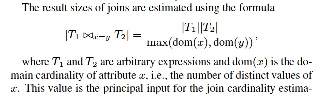
上面的公式需要满足下面3个假设,
均匀分布假设,所以总row count/Cardinality,才等于每个值的row count;
独立假设,所以T1和T2 join的空间为直接相乘,如果有相关性,空间就会变小
包含假设,所以取max,否则应该取并集,求并集的代价很高
To summarize, PostgreSQL’s cardinality estimator is based on the following assumptions:
uniformity: all values, except for the most-frequent ones, are assumed to have the same number of tuples
independence: predicates on attributes (in the same table or from joined tables) are independent
principle of inclusion: the domains of the join keys overlap such that the keys from the smaller domain have matches in the larger domain
The query engine of PostgreSQL takes a physical operator plan and executes it using Volcano-style interpretation.
The most important access paths are full table scans and lookups in unclustered B+Tree indexes.
Joins can be executed using either nested loops (with or without index lookups), in-memory hash joins, or sortmerge joins where the sort can spill to disk if necessary.
The decision which join algorithm is used is made by the optimizer and cannot be changed at runtime.
CARDINALITY ESTIMATION
Cardinality estimates are the most important ingredient for finding a good query plan.
Even exhaustive join order enumeration and a perfectly accurate cost model are worthless unless the cardinality estimates are (roughly) correct.
It is well known, however, that cardinality estimates are sometimes wrong by orders of magnitude, and that such errors are usually the reason for slow queries.
In this section, we experimentally investigate the quality of cardinality estimates in relational database systems by comparing the estimates with the true cardinalities.
Estimates for Base Tables
To measure the quality of base table cardinality estimates, we use the q-error, which is the factor by which an estimate differs from the true cardinality.
For example, if the true cardinality of an expression is 100, the estimates of 10 or 1000 both have a q-error of 10.
Using the ratio instead of an absolute or quadratic difference captures the intuition that for making planning decisions only relative differences matter.
The q-error furthermore provides a theoretical upper bound for the plan quality if the q-errors of a query are bounded [30].
Table 1 shows the 50th, 90th, 95th, and 100th percentiles of the q-errors for the 629 base table selections in our workload.
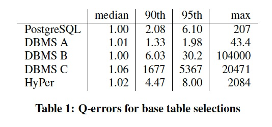
The median q-error is close to the optimal value of 1 for all systems, indicating that the majority of all selections are estimated correctly. 中位数接近1,表示这个场景对于大部分查询可以预估的比较准确
However, all systems produce misestimates for some queries, and the quality of the cardinality estimates differs strongly between the different systems.
Looking at the individual selections, we found that DBMS A and HyPer can usually predict even complex predicates like substring search using LIKE very well.
To estimate the selectivities for base tables HyPer uses a random sample of 1000 rows per table and applies the predicates on that sample. HyPer的方式是每个表1000行的抽样,一般情况下准确率比较高,但是对选择率比较低的误差会很大
This allows one to get accurate estimates for arbitrary base table predicates as long as the selectivity is not too low.
When we looked at the selections where DBMS A and HyPer produce errors above 2, we found that most of them have predicates with extremely low true selectivities.
This routinely happens when the selection yields zero tuples on the sample, and the system falls back on an ad-hoc estimation method (“magic constants”). 因为当选择率比较低的时候,大概率会在sampl的时候miss,导致退化成临时估计方式
It therefore appears to be likely that DBMS A also uses the sampling approach.
The estimates of the other systems are worse and seem to be based on per-attribute histograms, which do not work well for many predicates and cannot detect (anti-)correlations between attributes. 其他系统用的是单列Histogram,表现会差于Hyper的抽样,因为无法感知列关联
Note that we obtained all estimates using the default settings after running the respective statistics gathering tool.
Some commercial systems support the use of sampling for base table estimation, multi-attribute histograms (“column group statistics”), or ex post feedback from previous query runs [38]. 因为用的是默认配置,很多商业数据库的高级功能未打开
However, these features are either not enabled by default or are not fully automatic.
Estimates for Joins
Let us now turn our attention to the estimation of intermediate results for joins, which are more challenging because sampling or histograms do not work well.
Figure 3 summarizes over 100,000 cardinality estimates in a single figure.
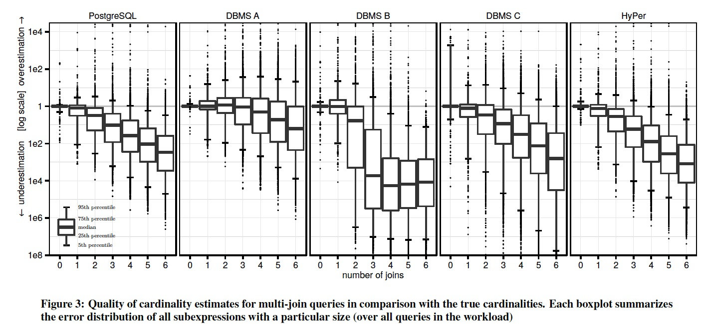
For each intermediate result of our query set, we compute the factor by which the estimate differs from the true cardinality, distinguishing between over- and underestimation.
The graph shows one “boxplot” (note the legend (说明)in the bottom-left corner) for each intermediate result size, 箱型图也是用于表现分位数的
which allows one to compare how the errors change as the number of joins increases.
The vertical axis uses a logarithmic scale(对数比例) to encompass underestimates by a factor of 108 and overestimates by a factor of 104.
Despite the better base table estimates of DBMS A, the overall variance of the join estimation errors, as indicated by the boxplot, is similar for all systems with the exception of DBMS B.
For all systems we routinely observe misestimates by a factor of 1000 or more.
Furthermore, as witnessed by the increasing height of the box plots, the errors grow exponentially (note the logarithmic scale) as the number of joins increases [21]. 当Join数变多的时候,errors呈指数级别增长
For PostgreSQL 16% of the estimates for 1 join are wrong by a factor of 10 or more. This percentage increases to 32% with 2 joins, and to 52% with 3 joins.
For DBMS A, which has the best estimator of the systems we compared, the corresponding percentages are only marginally better at 15%, 25%, and 36%.
Another striking observation is that all tested systems—though DBMS A to a lesser degree—tend to systematically underestimate the results sizes of queries with multiple joins. 所有系统在多表join时,会系统性的低估Cardinality
This can be deduced from the median of the error distributions in Figure 3.
For our query set, it is indeed the case that the intermediate results tend to decrease with an increasing number of joins because more base table selections get applied.
However, the true decrease is less than the independence assumption used by PostgreSQL (and apparently by the other systems) predicts.
Underestimation is most pronounced with DBMS B, which frequently estimates 1 row for queries with more than 2 joins.
The estimates of DBMS A, on the other hand, have medians that are much closer to the truth, despite their variance being similar to some of the other systems.
We speculate(guess) that DBMS A uses a damping factor(阻尼) that depends on the join size, similar to how many optimizers combine multiple selectivities. DBMS A看上去随着join数增加,误差变化没那么大,应该是简单的根据join数乘上一定的阻尼因子
Many estimators combine the selectivities of multiple predicates (e.g., for a base relation or for a subexpression with multiple joins) not by assuming full independence,
but by adjusting the selectivities “upwards”, using a damping factor.
The motivation for this stems from the fact that the more predicates need to be applied, the less certain one should be about their independence.
Given the simplicity of PostgreSQL’s join estimation formula (cf. Section 2.3) and the fact that its estimates are nevertheless competitive with the commercial systems,
we can deduce that the current join size estimators are based on the independence assumption. No system tested was able to detect join-crossing correlations. 和PG的对比,可以发现商业数据库系统的join size的预估并没有明显占优,所以也应该是基于独立假设,无法考虑到相关性
Furthermore, cardinality estimation is highly brittle(脆弱的,crisp), as illustrated by the significant number of extremely large errors we observed (factor 1000 or more) and the following anecdote(轶事):
In PostgreSQL, we observed different cardinality estimates of the same simple 2-join query depending on the syntactic order of the relations in the from and/or the join predicates in the where clauses!
Simply by swapping predicates or relations, we observed the estimates of 3, 9, 128, or 310 rows for the same query (with a true cardinality of 2600)6. 语法顺序也会大幅的改变预估值,简单的调换谓词和关系的顺序,得到的预估有较大的差异
Note that this section does not benchmark the query optimizers of the different systems.
In particular, our results do not imply that the DBMS B’s optimizer or the resulting query performance is necessarily worse than that of other systems, despite larger errors in the estimator.
The query runtime heavily depends on how the system’s optimizer uses the estimates and how much trust it puts into these numbers. Cardinality Estimator并不绝对决定优化器效果的好坏,还要看优化器如何使用CE的结果
A sophisticated engine may employ adaptive operators (e.g., [4, 8]) and thus mitigate the impact of misestimations.
The results do, however, demonstrate that the state-of-the-art in cardinality estimation is far from perfect.
Better Statistics for PostgreSQL
As mentioned in Section 2.3, the most important statistic for join estimation in PostgreSQL is the number of distinct values. 在Join estimation中最重要的指标是distinct values
These statistics are estimated from a fixed-sized sample, and we have observed severe underestimates for large tables. 在PG中distinct本身是通过固定大小的sample估计的,所以对于大表存在严重的underestimates
To determine if the misestimated distinct counts are the underlying problem for cardinality estimation,
we computed these values precisely and replaced the estimated with the true values. 在PG中,为了验证distinct的误差本身到底对join estimation的影响,我们用正确的精确值去替代错误值。
Figure 5 shows that the true distinct counts slightly improve the variance of the errors.
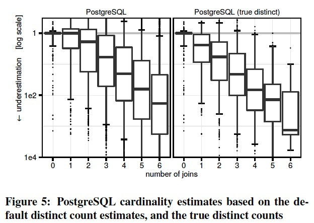
Surprisingly, however, the trend to underestimate cardinalities becomes even more pronounced(明显的). 但是将distinct换成精确值后,Cardinality预估的低估更加明显了
The reason is that the original, underestimated distinct counts resulted in higher estimates, which, accidentally, are closer to the truth. 因为较小的distinct会导致,每个值对应的row count变大,反而抵消了部分后续由于独立性假设带来的低估
This is an example for the proverbial(谚语的) “two wrongs that make a right”, i.e., two errors that (partially) cancel each other out.
Such behavior makes analyzing and fixing query optimizer problems very frustrating(令人沮丧的) because fixing one query might break another.
WHEN DO BAD CARDINALITY ESTIMATES LEAD TO SLOW QUERIES?
较大的Estimation的误差,由于各种原因不一定会导致慢查询,本章节重点分析各种情况下,estimation的误差会导致慢查询。
While the large estimation errors shown in the previous section are certainly sobering(清醒的), large errors do not necessarily lead to slow query plans.
For example, the misestimated expression may be cheap in comparison with other parts of the query,
or the relevant plan alternative may have been misestimated by a similar factor thus “canceling out” the original error.
In this section we investigate the conditions under which bad cardinalities are likely to cause slow queries.
查询优化的效果和索引的多少有较大的关系,所以分别讨论两种情况,仅有主键索引和多种索引的情况下
One important observation is that query optimization is closely intertwined with the physical database design:
the type and number of indexes heavily influence the plan search space, and therefore affects how sensitive the system is to cardinality misestimates.
We therefore start this section with experiments using a relatively robust physical design with only primary key indexes and
show that in such a setup the impact of cardinality misestimates can largely be mitigated.
After that, we demonstrate that for more complex configurations with many indexes, cardinality misestimation makes it much more likely to miss the optimal plan by a large margin(大幅的).
The Risk of Relying on Estimates
将不同的系统的estimation注入到PG中执行,看看对于查询执行的影响,这样可以隔离的看出,estimation对于整个查询的影响
虽然estimation的影响不是绝对的,但是在存在误差时,仍然在大部分情况下会影响到查询性能,并且在偶尔的情况下会导致timeout
To measure the impact of cardinality misestimation on query performance we injected the estimates of the different systems into PostgreSQL and then executed the resulting plans.
Using the same query engine allows one to compare the cardinality estimation components in isolation by (largely) abstracting away from the different query execution engines.
Additionally, we inject the true cardinalities, which computes the—with respect to the cost model—optimal plan.
A small number of queries become slightly slower using the true instead of the erroneous cardinalities.
This effect is caused by cost model errors, which we discuss in Section 5.
However, as expected, the vast majority of the queries are slower when estimates are used.
Using DBMS A’s estimates, 78% of the queries are less than 2 slower than using the true cardinalities, while for DBMS B this is the case for only 53% of the queries.
This corroborates(证实) the findings about the relative quality of cardinality estimates in the previous section.
Unfortunately, all estimators occasionally(偶尔) lead to plans that take an unreasonable time and lead to a timeout.
Surprisingly, however, many of the observed slowdowns are easily avoidable despite the bad estimates as we show in the following.
实际发现哪些超时的都是因为PG的优化器选择了nest loop join,因为estimation低估,倒是优化器从cost上判断用nl join的cost更低。
后面的实验证明,只要nl join disable掉,就能避免这种极坏的case,也就是说nl join完全没有存在的必要。
When looking at the queries that did not finish in a reasonable time using the estimates, we found that most have one thing in common:
PostgreSQL’s optimizer decides to introduce a nestedloop join (without an index lookup) because of a very low cardinality estimate, whereas in reality the true cardinality is larger.
As we saw in the previous section, systematic underestimation happens very frequently, which occasionally results in the introduction of nested-loop joins.
The underlying reason why PostgreSQL chooses nested-loop joins is that it picks the join algorithm on a purely cost-based basis.
For example, if the cost estimate is 1,000,000 with the nested-loop join algorithm and 1,000,001 with a hash join,
PostgreSQL will always prefer the nested-loop algorithm even if there is a equality join predicate, which allows one to use hashing.
Of course, given the O(n2) complexity of nested-loop join and O(n) complexity of hash join, and given the fact that underestimates are quite frequent, this decision is extremely risky.
And even if the estimates happen to be correct, any potential performance advantage of a nested-loop join in comparison with a hash join is very small, so taking this high risk can only result in a very small payoff(收益).
Therefore, we disabled nested-loop joins (but not index-nestedloop joins) in all following experiments.
As Figure 6b shows, when rerunning all queries without these risky nested-loop joins, we observed no more timeouts despite using PostgreSQL’s estimates.
Also, none of the queries performed slower than before despite having less join algorithm options, confirming our hypothesis that nested-loop joins (without indexes) seldom have any upside.
仍然有部分慢10倍以上的case,是因为PG9.4使用estimation来初始化hashjoin的内存中的hash table,由于estimation低估导致hashtable太小,这样冲突链过长,导致hash变成遍历
9.5解决这个问题,会根据实际行数来改变hash table的大小,这样可以解决这个问题,加上disable nl join,仅仅4%的查询和正确的estimation比慢2倍以上
However, this change does not solve all problems, as there are still a number of queries that are more than a factor of 10 slower (慢10倍以上)(cf., red bars) in comparison with the true cardinalities.
When investigating the reason why the remaining queries still did not perform as well as they could, we found that most of them contain a hash join where the size of the build input is underestimated.
PostgreSQL up to and including version 9.4 chooses the size of the in-memory hash table based on the cardinality estimate.
Underestimates can lead to undersized hash tables with very long collisions chains and therefore bad performance.
The upcoming version 9.5 resizes the hash table at runtime based on the number of rows actually stored in the hash table.
We backported this patch to our code base, which is based on 9.4, and enabled it for all remaining experiments.
Figure 6c shows the effect of this change in addition with disabled nested-loop joins.
Less than 4% of the queries are off by more than 2 in comparison with the true cardinalities.
总结下,单纯CBO是不行的,存在一定的不确定性,需要做一些限制和约束
To summarize, being “purely cost-based”, i.e., not taking into account the inherent uncertainty of cardinality estimates
and the asymptotic complexities of different algorithm choices, can lead to very bad query plans.
Algorithms that seldom offer a large benefit over more robust algorithms should not be chosen.
Furthermore, query processing algorithms should, if possible, automatically determine their parameters at runtime instead of relying on cardinality estimates.
Good Plans Despite Bad Cardinalities
虽然不同的join order会导致数个量级的性能差异。
但是当只有主键索引的时候,Bad Cardinality和Good之间对性能的影响不大。因为哪怕Bad Cardinality也足够避免极坏的case,而其他case都需要做事实表的scan。
The query runtimes of plans with different join orders often vary by many orders of magnitude (cf. Section 6.1).
Nevertheless, when the database has only primary key indexes, as in all in experiments so far,
and once nested loop joins have been disabled and rehashing has been enabled, the performance of most queries is close to the one obtained using the true cardinalities.
Given the bad quality of the cardinality estimates, we consider this to be a surprisingly positive result. It is worthwhile to reflect on why this is the case.
The main reason is that without foreign key indexes, most large (“fact”) tables need to be scanned using full table scans, which dampens(抑制) the effect of different join orders.
The join order still matters, but the results indicate that the cardinality estimates are usually good enough to rule out all disastrous join order decisions like joining two large tables using an unselective join predicate.
Another important reason is that in main memory picking an index nested-loop join where a hash join would have been faster is never disastrous.
With all data and indexes fully cached, we measured that the performance advantage of a hash join over an index-nestedloop join is at most 5* with PostgreSQL and 2* with HyPer.
Obviously, when the index must be read from disk, random IO may result in a much larger factor. Therefore, the main-memory setting is much more forgiving.
Complex Access Paths
如果加上很多索引的情况下,由Bad Cardinality的join order问题会对查询性能产生更显著的影响
So far, all query executions were performed on a database with indexes on primary key attributes only.
To see if the query optimization problem becomes harder when there are more indexes, we additionally indexed all foreign key attributes.
Figure 7b shows the effect of additional foreign key indexes.
We see large performance differences with 40% of the queries being slower by a factor of 2!
Note that these results do not mean that adding more indexes decreases performance (although this can occasionally happen).
Indeed overall performance generally increases significantly, but the more indexes are available the harder the job of the query optimizer becomes.
Join-Crossing Correlations
在有关联查询谓词的情况下的中间结果Cardinality的预估是查询优化的前沿。
对于单表的关联谓词的预估,通过sample就可以达到比较好的效果,比如Hyper
但对于多表谓词关联性,很难有效的sample,所以比较困难,这类问题称为,join-cross correlations。
这里举了一个例子,没有给出通用的方法
There is consensus(共识) in our community that estimation of intermediate result cardinalities in the presence of (在。。。存在)correlated query predicates is a frontier(前沿) in query optimization research.
The JOB workload studied in this paper consists of real-world data and its queries contain many correlated predicates.
Our experiments that focus on single-table subquery cardinality estimation quality (cf. Table 1)
show that systems that keep table samples (HyPer and presumably DBMS A) can achieve almost perfect estimation results, even for correlated predicates (inside the same table).
As such, the cardinality estimation research challenge appears to lie in queries where the correlated predicates involve columns from different tables, connected by joins.
These we call “join-crossing correlations”.
Such correlations frequently occur in the IMDB data set, e.g., actors born in Paris are likely to play in French movies.
Given these join-crossing correlations one could wonder if there exist complex access paths that allow to exploit these.
One example relevant here despite its original setting in XQuery processing is ROX [22].
It studied runtime join order query optimization in the context of DBLP co-authorship queries that count how many Authors had published Papers in three particular venues, out of many.
These queries joining the author sets from different venues clearly have join-crossing correlations, since authors who publish
in VLDB are typically database researchers, likely to also publish in SIGMOD, but not—say—in Nature.
In the DBLP case, Authorship is a n : m relationship that links the relation Authors with the relation Papers.
The optimal query plans in [22] used an index-nested-loop join, looking up each author into Authorship.author (the indexed primary key) followed by a filter restriction on Paper.venue,
which needs to be looked up with yet another join.
This filter on venue would normally have to be calculated after these two joins.
However, the physical design of [22] stored Authorship partitioned by Paper.venue.7
This partitioning has startling(令人吃惊的) effects: instead of one Authorship table and primary key index, one physically has many, one for each venue partition.
This means that by accessing the right partition, the filter is implicitly enforced (for free), before the join happens.
This specific physical design therefore causes the optimal plan to be as follows:
first join the smallish authorship set from SIGMOD with the large set for Nature producing almost no result tuples, making the subsequent nested-loops index lookup join into VLDB very cheap.
If the tables would not have been partitioned, index lookups from all SIGMOD authors into Authorships would first find all co-authored papers,
of which the great majority is irrelevant because they are about database research, and were not published in Nature.
Without this partitioning, there is no way to avoid this large intermediate result, and there is no query plan that comes close to the partitioned case in efficiency:
even if cardinality estimation would be able to predict join-crossing correlations, there would be no physical way to profit from this knowledge.
The lesson to draw from this example is that the effects of query optimization are always gated by the available options in terms of access paths.
Having a partitioned index on a join-crossing predicate as in [22] is a non-obvious physical design alternative
which even modifies the schema by bringing in a join-crossing column (Paper.venue) as partitioning key of a table (Authorship).
The partitioned DBLP set-up is just one example of how one particular join-crossing correlation can be handled, rather than a generic solution.
Join-crossing correlations remain an open frontier for database research involving the interplay of physical design, query execution and query optimization.
In our JOB experiments we do not attempt to chart this mostly unknown space,
but rather characterize the impact of (join-crossing) correlations on the current stateof- the-art of query processing, restricting ourselves to standard PK and FK indexing.
COST MODELS
The cost model guides the selection of plans from the search space.
The cost models of contemporary(当代的) systems are sophisticated software artifacts(人工产物) that are resulting from 30+ years of research and development,
mostly concentrated in the area of traditional disk-based systems.
PostgreSQL’s cost model, for instance, is comprised(包含) of over 4000 lines of C code, and takes into account various subtle(微妙的) considerations,
e.g., it takes into account partially correlated index accesses, interesting orders, tuple sizes, etc.
It is interesting, therefore, to evaluate how much a complex cost model actually contributes to the overall query performance.
First, we will experimentally establish the correlation between the PostgreSQL cost model—a typical cost model of a disk-based DBMS—and the query runtime.
Then, we will compare the PostgreSQL cost model with two other cost functions.
The first cost model is a tuned version of PostgreSQL’s model for a main-memory setup where all data fits into RAM.
The second cost model is an extremely simple function that only takes the number of tuples produced during query evaluation into account.
We show that, unsurprisingly, the difference between the cost models is dwarfed(相形见绌) by the cardinality estimates errors.
We conduct our experiments on a database instance with foreign key indexes.
We begin with a brief description of a typical disk-oriented complex cost model, namely the one of PostgreSQL.
The PostgreSQL Cost Model
PG的cost模型,基于CPU和IO的加权的计算,其中weight和参数是由设计者规定的。并且PG不建议更改,会有比较大的风险。
PostgreSQL’s disk-oriented cost model combines CPU and I/O costs with certain weights.
Specifically, the cost of an operator is defined as a weighted sum of the number of accessed disk pages (both sequential and random) and the amount of data processed in memory.
The cost of a query plan is then the sum of the costs of all operators.
The default values of the weight parameters used in the sum (cost variables) are set by the optimizer designers
and are meant to reflect the relative difference between random access, sequential access and CPU costs.
The PostgreSQL documentation contains the following note on cost variables:
“Unfortunately, there is no well-defined method for determining ideal values for the cost variables.
They are best treated as averages over the entire mix of queries that a particular installation will receive.
This means that changing them on the basis of just a few experiments is very risky.”
For a database administrator, who needs to actually set these parameters these suggestions are not very helpful;
no doubt most will not change these parameters.
This comment is of course, not PostgreSQL-specific, since other systems feature similarly complex cost models.
In general, tuning and calibrating(标定) cost models (based on sampling, various machine learning techniques etc.) has been a subject of a number of papers (e.g, [42, 25]).
It is important, therefore, to investigate the impact of the cost model on the overall query engine performance.
This will indirectly show the contribution of cost model errors on query performance.
Cost and Runtime
这章主要讨论Cost模型对于查询优化的影响
结论从下面的图就比较清晰的看出来,
cost model上分为3种,PG原生的;针对当前硬件演进,降低process和读page的cost比例;简单模型,直接用row count,不考虑io,cpu
同时在Cardinality上,分布使用estimation和true。
图上明显可见,Cardinality变成true对于提升cost的准确性作用是非常明显的,而改进或简化cost模型本身是对cost的准确性提升非常有限。
这里我对于这个结论持怀疑,有一定局限
因为本身PG的模型就不是非常的复杂或是精确,所以你无论是做小的调整或简化,自然不会有太大的变化。并且对于传统的数据库,其实row count本身确实就可以代表大部分的cost。
The main virtue of a cost function is its ability to predict which of the alternative query plans will be the fastest, given the cardinality estimates;
in other words, what counts is its correlation with the query runtime.
The correlation between the cost and the runtime of queries in PostgreSQL is shown in Figure 8a.

Additionally, we consider the case where the engine has the true cardinalities injected, and plot the corresponding data points in Figure 8b.
For both plots, we fit the linear regression model (displayed as a straight line) and highlight the standard error.
The predicted cost of a query correlates with its runtime in both scenarios.
Poor cardinality estimates, however, lead to a large number of outliers and a very wide standard error area in Figure 8a.
Only using the true cardinalities makes the PostgreSQL cost model a reliable predictor of the runtime, as has been observed previously [42].
Intuitively, a straight line in Figure 8 corresponds to an ideal cost model that always assigns (predicts) higher costs for more expensive queries.
Naturally, any monotonically increasing function would satisfy that requirement, but the linear model provides the simplest and the closest fit to the observed data.
We can therefore interpret the deviation from this line as the prediction error of the cost model.
Specifically, we consider the absolute percentage error of a cost model for a query Q: (Q) = (real(Q) - pred(Q)) / real(Q) ,
where real is the observed runtime, and pred is the runtime predicted by our linear model.
Using the default cost model of PostgreSQL and the true cardinalities, the median error of the cost model is 38%.
Tuning the Cost Model for Main Memory
As mentioned above, a cost model typically involves parameters that are subject to tuning by the database administrator.
In a disk-based system such as PostgreSQL, these parameters can be grouped into CPU cost parameters and I/O cost parameters,
with the default settings reflecting an expected proportion between these two classes in a hypothetical workload.
In many settings the default values are sub optimal.
For example, the default parameter values in PostgreSQL suggest that processing a tuple is 400x cheaper than reading it from a page.
However, modern servers are frequently equipped with very large RAM capacities,
and in many workloads the data set actually fits entirely into available memory (admittedly(诚然), the core of PostgreSQL was shaped decades ago when database servers only had few megabytes of RAM).
This does not eliminate the page access costs entirely (due to buffer manager overhead), but significantly bridges the gap between the I/O and CPU processing costs.
Arguably, the most important change that needs to be done in the cost model for a main-memory workload is to decrease the proportion between these two groups.
We have done so by multiplying the CPU cost parameters by a factor of 50.
The results of the workload run with improved parameters are plotted in the two middle subfigures of Figure 8.
Comparing Figure 8b with d, we see that tuning does indeed improve the correlation between the cost and the runtime.
On the other hand, as is evident from comparing Figure 8c and d, parameter tuning improvement is still overshadowed(黯然失色) by the difference between the estimated and the true cardinalities.
Note that Figure 8c features a set of outliers for which the optimizer has accidentally discovered very good plans (runtimes around 1 ms) without realizing it (hence very high costs).
This is another sign of “oscillation” in query planning caused by cardinality misestimates.
In addition, we measure the prediction error of the tuned cost model, as defined in Section 5.2.
We observe that tuning improves the predictive power of the cost model: the median error decreases from 38% to 30%.
Are Complex Cost Models Necessary?
As discussed above, the PostgreSQL cost model is quite complex.
Presumably(想必), this complexity should reflect various factors influencing query execution, such as the speed of a disk seek and read, CPU processing costs, etc.
In order to find out whether this complexity is actually necessary in a main-memory setting, we will contrast it with a very simple cost function Cmm.
This cost function is tailored for the main-memory setting in that it does not model I/O costs, but only counts the number of tuples that pass through each operator during query execution:
The results of our workload run with Cmm as a cost function are depicted in Figure 8e and f.
We see that even our trivial cost model is able to fairly accurately predict the query runtime using the true cardinalities.
To quantify this argument, we measure the improvement in the runtime achieved by changing the cost model for true cardinalities:
In terms of the geometric mean over all queries, our tuned cost model yields 41% faster runtimes than the standard PostgreSQL model,
but even a simple Cmm makes queries 34% faster than the built-in cost function.
This improvement is not insignificant, but on the other hand, it is dwarfed by improvement in query runtime observed when we replace estimated cardinalities with the real ones (cf. Figure 6b).
This allows us to reiterate our main message that cardinality estimation is much more crucial than the cost model.
PLAN SPACE
Besides cardinality estimation and the cost model, the final important query optimization component is a plan enumeration algorithm that explores the space of semantically equivalent join orders.
Many different algorithms, both exhaustive (e.g., [29, 12]) as well as heuristic (e.g, [37, 32]) have been proposed.
These algorithms consider a different number of candidate solutions (that constitute the search space) when picking the best plan.
In this section we investigate how large the search space needs to be in order to find a good plan.
针对两种思路,实现了一种DP的穷尽算法,或若干启发式的算法。
这里由于数量太大,直接用true Cardinality和cost模型算出的cost来模拟真实执行时间,从上一章结论来看,这是reasonable的
The experiments of this section use a standalone query optimizer, which implements Dynamic Programming (DP) and a number of heuristic join enumeration algorithms.
Our optimizer allows the injection of arbitrary cardinality estimates.
In order to fully explore the search space, we do not actually execute the query plans produced by the optimizer in this section, as that would be infeasible due to the number of joins our queries have.
Instead, we first run the query optimizer using the estimates as input.
Then, we recompute the cost of the resulting plan with the true cardinalities, giving us a very good approximation of the runtime the plan would have in reality.
We use the in-memory cost model from Section 5.4 and assume that it perfectly predicts the query runtime,
which, for our purposes, is a reasonable assumption since the errors of the cost model are negligible(微不足道) in comparison the cardinality errors.
This approach allows us to compare a large number of plans without executing all of them.
How Important Is the Join Order?
这里的实验只是说明,Join Order对于join的执行效果的影响是数个量级的,并且在无index或是PK的情况下,差别在100倍左右,但是当具有PK+FK的时候,差别达到万的级别。
We use the Quickpick [40] algorithm to visualize the costs of different join orders.
Quickpick is a simple, randomized algorithm that picks joins edges at random until all joined relations are fully connected.
Each run produces a correct, but usually slow, query plan.
By running the algorithm 10,000 times per query and computing the costs of the resulting plans, we obtain an approximate distribution for the costs of random plans.
Figure 9 shows density plots for 5 representative example queries and for three physical database designs: no indexes, primary key indexes only, and primary+foreign key indexes.
The costs are normalized by the optimal plan (with foreign key indexes), which we obtained by running dynamic programming and the true cardinalities.
The graphs, which use a logarithmic scale on the horizontal cost axis, clearly illustrate the importance of the join ordering problem:
The slowest or even median cost is generally multiple orders of magnitude more expensive than the cheapest plan.
The shapes of the distributions are quite diverse.
For some queries, there are many good plans (e.g., 25c), for others few (e.g., 16d).
The distribution are sometimes wide (e.g., 16d) and sometimes narrow (e.g., 25c).
The plots for the “no indexes” and the “PK indexes” configurations are very similar implying that for our workload primary key indexes alone do not improve performance very much,
since we do not have selections on primary key columns.
In many cases the “PK+FK indexes” distributions have additional small peaks on the left side of the plot,
which means that the optimal plan in this index configuration is much faster than in the other configurations.
We also analyzed the entire workload to confirm these visual observations:
The percentage of plans that are at most 1:5 more expensive than the optimal plan is 44% without indexes, 39% with primary key indexes, but only 4% with foreign key indexes.
The average fraction between the worst and the best plan, i.e., the width of the distribution, is 101 without indexes, 115 with primary key indexes, and 48120 with foreign key indexes.
These summary statistics highlight the dramatically different search spaces of the three index configurations.
Are Bushy Trees Necessary?
比较三种树结构,表明zig zag要好于左深树
Most join ordering algorithms do not enumerate all possible tree shapes.
Virtually all optimizers ignore join orders with cross products, which results in a dramatically reduced optimization time with only negligible query performance impact.
Oracle goes even further by not considering bushy join trees [1].
In order to quantify the effect of restricting the search space on query performance, we modified our DP algorithm to only enumerate left-deep, right-deep, or zig-zag trees.
Aside from the obvious tree shape restriction, each of these classes implies constraints on the join method selection.
We follow the definition by Garcia-Molina et al.’s textbook, which is reverse from the one in Ramakrishnan and Gehrke’s book:
Using hash joins, right-deep trees are executed by first creating hash tables out of each relation except one before probing in all of these hash tables in a pipelined fashion,
whereas in left-deep trees, a new hash table is built from the result of each join.
In zig-zag trees, which are a super set of all left- and right-deep trees, each join operator must have at least one base relation as input.
For index-nested loop joins we additionally employ the following convention:
the left child of a join is a source of tuples that are looked up in the index on the right child, which must be a base table.
Using the true cardinalities, we compute the cost of the optimal plan for each of the three restricted tree shapes.
We divide these costs by the optimal tree (which may have any shape, including “bushy”) thereby measuring how much performance is lost by restricting the search space.
The results in Table 2 show that zig-zag trees offer decent(好的) performance in most cases, with the worst case being 2:54 more expensive than the best bushy plan.
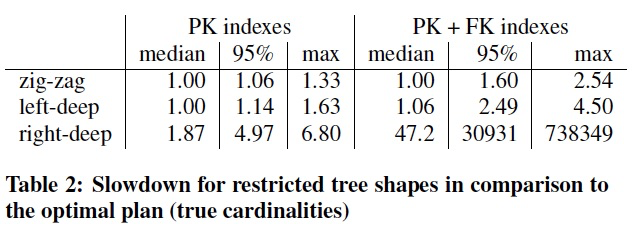
Left-deep trees are worse than zig-zag trees, as expected, but still result in reasonable performance.
Right-deep trees, on the other hand, perform much worse than the other tree shapes and thus should not be used exclusively.
The bad performance of right-deep trees is caused by the large intermediate hash tables that need to be created from each base relation
and the fact that only the bottom-most join can be done via index lookup.
Are Heuristics Good Enough?
启发式的search算法已经足够好了,其实这里主要是要可以屏蔽掉最坏的查询,即可,故无必要做DP穷举;仍然表明统计信息的准确是更为关键的
所以问题在于如果高效的优化器中实现启发式算法来balance
So far in this paper, we have used the dynamic programming algorithm, which computes the optimal join order.
However, given the bad quality of the cardinality estimates, one may reasonably ask whether an exhaustive algorithm is even necessary.
We therefore compare dynamic programming with a randomized and a greedy heuristics.
The “Quickpick-1000” heuristics is a randomized algorithm that chooses the cheapest (based on the estimated cardinalities) 1000 random plans.
Among all greedy heuristics, we pick Greedy Operator Ordering (GOO) since it was shown to be superior to other deterministic approximate algorithms [11].
GOO maintains a set of join trees, each of which initially consists of one base relation.
The algorithm then combines the pair of join trees with the lowest cost to a single join tree.
Both Quickpick-1000 and GOO can produce bushy plans, but obviously only explore parts of the search space.
All algorithms in this experiment internally use the PostgreSQL cardinality estimates to compute a query plan,
for which we compute the “true” cost using the true cardinalities.
Table 3 shows that it is worthwhile to fully examine the search space using dynamic programming despite cardinality misestimation.
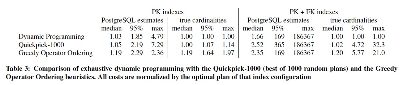
However, the errors introduced by estimation errors cause larger performance losses than the heuristics.
In contrast to some other heuristics (e.g., [5]), GOO and Quickpick-1000 are not really aware of indexes.
Therefore, GOO and Quickpick-1000 work better when few indexes are available, which is also the case when there are more good plans.
To summarize, our results indicate that enumerating all bushy trees exhaustively offers moderate but not insignificant performance benefits
in comparison with algorithms that enumerate only a sub set of the search space.
The performance potential from good cardinality estimates is certainly much larger.
However, given the existence of exhaustive enumeration algorithms that can find the optimal solution for queries with dozens of relations very quickly (e.g.,
[29, 12]), there are few cases where resorting to heuristics or disabling bushy trees should be necessary.
RELATED WORK
Our cardinality estimation experiments show that systems which keep table samples for cardinality estimation predict single-table result sizes
considerably better than those which apply the independence assumption and use single-column histograms [20]. 对于单表的CE,Sample的效果会远好于采用独立假设的单列Histogram
We think systems should be adopting table samples as a simple and robust technique,
rather than earlier suggestions to explicitly detect certain correlations [19] to subsequently create multi-column histograms [34] for these. 故不建议采用多列histograms的方式来表示列相关性
However, many of our JOB queries contain join-crossing correlations, which single-table samples do not capture, 现在的系统对于跨表的join-crossing相关性,由于通过单表sample无法capture,仍然采用独立假设的方式
and where the current generation of systems still apply the independence assumption.
There is a body of existing research work to better estimate result sizes of queries with join-crossing correlations,
mainly based on join samples [17], possibly enhanced against skew (endbiased sampling [10], correlated samples [43]), using sketches [35] or graphical models [39].
This work confirms that without addressing join-crossing correlations, cardinality estimates deteriorate(恶化) strongly with more joins [21], leading to both the over- and underestimation of result sizes (mostly the latter),
so it would be positive if some of these techniques would be adopted by systems. Research工作中提出一些方法来解决join-crossing的问题,证明当前的独立假设会导致误差随join个数变多而持续恶化,如果这些方法能够被实现,应该对于问题会有所帮助
Another way of learning about join-crossing correlations is by exploiting query feedback, as in the LEO project [38],
though there it was noted that deriving cardinality estimations based on a mix of exact knowledge and lack of knowledge needs a sound(良好) mathematical underpinning(基础).
For this, maximum entropy (MaxEnt [28, 23]) was defined, though the costs for applying maximum entropy are high and have prevented its use in systems so far.
We found that the performance impact of estimation mistakes heavily depends on the physical database design;
in our experiments the largest impact is in situations with the richest designs.
From the ROX [22] discussion in Section 4.4 one might conjecture that to truly unlock the potential of correctly predicting cardinalities for join-crossing correlations, we also need new physical designs and access paths.
由于CE的不准确,所以如果采用对冲的策略,即不一定要选择cheapest的plan,而是要尽量避免高风险的plan,哪怕他们在cost上更低
Another finding in this paper is that the adverse effects(不利的) of cardinality misestimations can be strongly reduced if systems would be “hedging their bets(对冲赌注)” and not only choose the plan with the cheapest expected cost,
but take the probabilistic distribution of the estimate into account, to avoid plans that are marginally(略,稍微) faster than others but bear a high risk of strong underestimation.
There has been work both on doing this for cardinality estimates purely [30], as well as combining these with a cost model (cost distributions [2]).
The problem with fixed hash table sizes for PostgreSQL illustrates that cost misestimation can often be mitigated(缓解) by making the runtime behavior of the query engine more “performance robust”.
This links to a body of work to make systems adaptive to estimation mistakes, e.g., dynamically switch sides in a join, or change between hashing and sorting (GJoin [15]),
switch between sequential scan and index lookup (smooth scan [4]), adaptively reordering join pipelines during query execution [24],
or change aggregation strategies at runtime depending on the actual number of group-by values [31] or partition-by values [3].
A radical(激进的) approach is to move query optimization to runtime, when actual value-distributions become available [33, 9].
However, runtime techniques typically restrict the plan search space to limit runtime plan exploration cost, 当具有实际的数据分布时,可以采用激进的RunTime方法,这种方式会限制搜索空间和access paths
and sometimes come with functional restrictions such as to only consider (sampling through) operators which have pre-created indexed access paths (e.g., ROX [22]).
Our experiments with the second query optimizer component besides cardinality estimation, namely the cost model, suggest that tuning cost models provides less benefits than improving cardinality estimates,
and in a main-memory setting even an extremely simple cost-model can produce satisfactory results.
This conclusion resonates(共鸣) with some of the findings in [42] which sets out(着手) to improve cost models but shows major improvements by refining cardinality estimates with additional sampling.
For testing the final query optimizer component, plan enumeration, we borrowed in our methodology from the Quickpick method used in randomized query optimization [40] to characterize and visualize the search space.
Another well-known search space visualization method is Picasso [18], which visualizes query plans as areas in a space where query parameters are the dimensions. 这里提到两个查询空间的visualize的方法,可以借鉴
Interestingly, [40] claims in its characterization of the search space that good query plans are easily found, but our tests indicate that the richer the physical design and access path choices, the rarer good query plans become.
Query optimization is a core database research topic with a huge body of related work, that cannot be fully represented in this section.
After decades of work still having this problem far from resolved [26], some have even questioned it and argued for the need of optimizer application hints [6].
This paper introduces the Join Order Benchmark based on the highly correlated IMDB real-world data set and a methodology for measuring the accuracy of cardinality estimation.
Its integration in systems proposed for testing and evaluating the quality of query optimizers [41, 16, 14, 27] is hoped to spur further innovation in this important topic.

 浙公网安备 33010602011771号