Python作业4：数据可视化

1、作业一

（1）作业要求

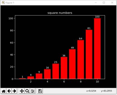
对下图进行修改：

1. 请更换图形的风格

2. 请将x轴的数据改为-10到10

3. 请自行构造一个y值的函数

4. 请将直方图上的数字，位置改到柱形图的内部垂直居中的位置

（2）作业分析与代码实现

1. 更换图形风格：

图形风格使用plt.style.use()语句实现，使用命令plt.style.available查看所有可用的风格如下：

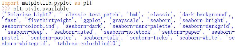
这里我选择风格'bmh'：

plt.style.use('bmh')

2. 将x轴的数据改为-10到10：

创建numpy数组x，以x作为横坐标，并把坐标步长改为1即可：

x = np.array([i for i in range(-10, 11)])
x_major_locator = MultipleLocator(2) # 把x轴的刻度间隔设置为2，并存在变量里
ax.xaxis.set_major_locator(x_major_locator) # 把x轴的主刻度设置为2的倍数

3. 自行构造y函数：

y = 2 * x * x + 2

4. 将直方图上的数字改到柱形图内部垂直居中的位置：

显示数据标签的函数：

plt.text(x, y, s, fontsize, verticalalignment,horizontalalignment,rotation , **kwargs)

其中x，y表示要显示标签的位置（坐标）；fontsize为标签字号大小；verticalalignment用va代表，表示垂直对齐方式，可选 'center' ，'top' ， 'bottom'，'baseline' 等；horizontalalignment用ha代表，表示水平对齐方式，可以填 'center' ， 'right' ，'left' 等。

所以要将标签改到柱形图内部垂直居中位置，则用以下语句即可：

plt.text(x, y / 2, y, ha = 'center', va = 'center', fontsize = 10)

5. 综合上述代码，可编写程序如下：

import numpy as np
import matplotlib.pyplot as plt
from matplotlib.pyplot import MultipleLocator

plt.style.use('bmh')     # 图像风格
fig, ax = plt.subplots()
fig.canvas.set_window_title('Homework 1')
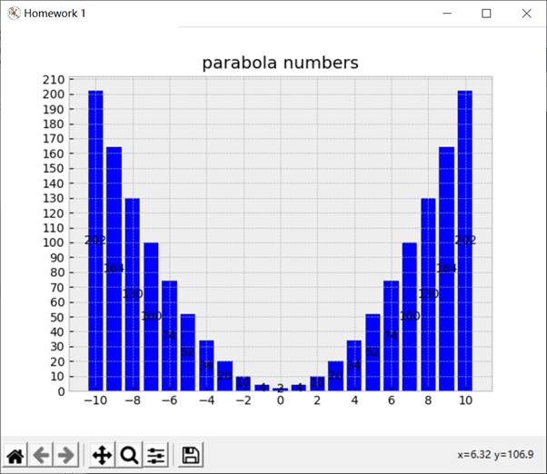
ax.set_title("parabola numbers")    # 标题
x = np.array([i for i in range(-10, 11)])
y = 2 * x * x + 2
plt.bar(x, y, color = 'b')      # bar颜色改为蓝色

x_major_locator = MultipleLocator(2)        # 把x轴的刻度间隔设置为1，并存在变量里
y_major_locator = MultipleLocator(10)       # 把y轴的刻度间隔设置为10，并存在变量里
ax.xaxis.set_major_locator(x_major_locator) # 把x轴的主刻度设置为1的倍数
ax.yaxis.set_major_locator(y_major_locator) # 把y轴的主刻度设置为10的倍数

for a, b in zip(x, y):
    """在直方图上显示数字"""
    plt.text(a, b / 2, '%d' % b, ha = 'center', va = 'center', fontsize = 10)

plt.show()

（3）效果演示

2、作业二

（1）作业要求

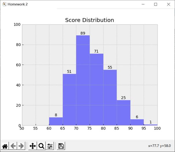
对成绩数据data1402.csv进行分段统计：每5分作为一个分数段，展示出每个分数段的人数直方图。

（2）作业分析与代码实现

1. 要统计每5分之间的人数，可以用到pyplot中频数直方图hist（万能的python，虽然也可以用普通bar实现，不过人生苦短，我用python）：

'plt.hist(scores, bins, alpha=0.5, histtype = 'stepfilled', color = 'b')'

参数分析：

• scores：要统计的数据

• bins：指定bin(箱子)的个数,也就是总共有几条条状图

• alpha：条状图透明度

• histtype：条状图填充形式，"stepfilled"即步长之间填充满

• color：条状图颜色

2. 先读取data1402.csv文件中的分数，存入列表scores；

3. 求每个区间的人数，以5为步长，构造函数countStep，判断分数所在区间用（分数 // 5 * 5）可以实现，以此得到字典类型：区间与人数的映射；

4. 综合上述分析，编写程序如下：

"""频数直方图"""

import csv
import numpy as np
import matplotlib.pyplot as plt
from matplotlib.pyplot import MultipleLocator
import pandas as pd

scores = []     # 列表对象
with open('data1402.csv', 'r') as csvFile:
    f_csv = csv.reader(csvFile)     # 读取文件
    for row in f_csv:
        """将每一行数据保存到scores中"""
        scores.append(int(float(row[0])))   # 因为文件中一行一个数字，所以row[0]


def countStep(scores):
    """求每个区间的人数，以5为步长，从50开始"""
    scoreCnt = {}
    for emp in scores:
        section = emp // 5 * 5        # 判断所在区间
        scoreCnt[section] = scoreCnt.get(section, 0) + 1
    return scoreCnt


counted = countStep(scores)      # 字典 = {分数 : 人数}

plt.style.use('bmh')     # 图像风格
fig, ax = plt.subplots()
fig.canvas.set_window_title('Homework 2')
ax.set_title("Score Distribution")    # 标题
# 设置x轴和y轴的最小值和最大值
xmin, xmax, ymin, ymax = 50, 100, 0, 100
plt.axis([xmin, xmax, ymin, ymax])
# 设置x轴区间，以5为步长
plt.xticks([x for x in range(xmin, xmax + 1) if x % 5 == 0])  # x标记step设置为5

# 绘制频次直方图，以5为步长
step = 5
bins = [x for x in range(xmin, xmax + 1, step)]
print(bins)
print(scores)
plt.hist(scores, bins, alpha=0.5, histtype='stepfilled', color='b')
for key in counted:
    """在直方图上显示数字"""
    plt.text(key + 2.5, counted.get(key, 0) + 0.2, '%d' % counted.get(key, 0), ha = 'center', va = 'bottom', fontsize = 10)

plt.show()

（3）效果演示

3、作业三

（1）作业要求

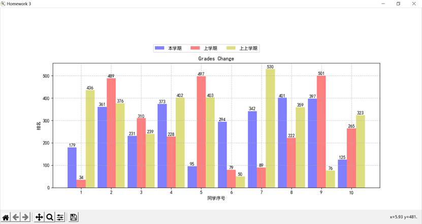
自行创建出10个学生的3个学期排名数据，并通过直方图进行对比展示。

（2）作业分析及代码实现

1. 自行创建10个学生的3个学期排名数据：使用随机数即可（所以排名跌宕起伏也不奇怪了），创建三个学期十名同学的排名列表：semester1、semester2、semester3；

2. 将一个同学的三个学期的排名放一起进行对比，每个条状图宽度0.3，则bar生成时，本学期的位置为x - 0.3、上学期为x、上上学期为x + 0.3： plt.bar(x - 0.3, semester1, 0.3, alpha = 0.5, color = 'b')

plt.bar(x, semester2, 0.3, alpha = 0.5, color = 'r')

plt.bar(x + 0.3, semester3, 0.3, alpha = 0.5, color = 'y')

3. 数据标签x坐标同直方图；

4. 设置图例：

box = ax.get_position()

ax.set_position([box.x0, box.y0, box.width , box.height* 0.8]) # 将图例放上面就box.height*0.8，放右边就box.width*0.8

ax.legend(['本学期', '上学期', '上上学期'], loc='center left', bbox_to_anchor = (0.3, 1.12), ncol = 3)

5. 综合上述分析，编写程序如下：

"""绘制三个对比直方图"""
import csv
import numpy as np
import matplotlib.pyplot as plt
from matplotlib.pyplot import MultipleLocator
import pandas as pd
from random import randint

fig = plt.figure(figsize=(10, 10))          # 窗口大小
fig.canvas.set_window_title('Homework 3')   # 窗口标题
ax = plt.axes()     # 创建坐标对象
ax.set_title("Grades Change")               # 直方图标题
ax.set_ylabel('排名')
ax.set_xlabel('同学序号')
plt.rcParams['font.sans-serif'] = ['SimHei']        # 添加对中文字体的支持
semester1 = []      # 保存第一学期的排名
semester2 = []      # 保存第二学期的排名
semester3 = []      # 保存第三学期的排名
for i in range(10):
    """生成10名同学三个学期的排名"""
    s1 = randint(1, 570)
    s2 = randint(1, 570)
    s3 = randint(1, 570)
    semester1.append(s1)
    semester2.append(s2)
    semester3.append(s3)


# 打印三学期成绩对比
for i in range(10):
    print(semester1[i], semester2[i], semester3[i])

# 创建两个直方图，注意它们在x轴的位置，不能重合
x = np.arange(1, 11)        # 生成横轴数据，10位同学
x_major_locator = MultipleLocator(1)       # 把y轴的刻度间隔设置为10，并存在变量里
ax.xaxis.set_major_locator(x_major_locator) # 把x轴的主刻度设置为1的倍数
# 生成本学期的排名直方图，宽度为0.3
plt.bar(x - 0.3, semester1, 0.3, alpha = 0.5, color = 'b')
# 生成上学期的排名直方图，上一个直方图向右0.3宽度
plt.bar(x, semester2, 0.3, alpha = 0.5, color = 'r')
# 生成上上学期的排名直方图，向右0.3宽度
plt.bar(x + 0.3, semester3, 0.3, alpha = 0.5, color = 'y')

for a, b in zip(x, semester1):
    """设置本学期排名标签"""
    plt.text(a - 0.3, b + 0.2, b, ha = 'center', va = 'bottom', fontsize = 10)
for a, b in zip(x, semester2):
    """设置上学期排名标签"""
    plt.text(a, b + 0.2, b, ha = 'center', va = 'bottom', fontsize = 10)
for a, b in zip(x, semester3):
    """设置上上学期排名标签"""
    plt.text(a + 0.3, b + 0.2, b, ha = 'center', va = 'bottom', fontsize = 10)

# 设置图例legend位置
box = ax.get_position()
ax.set_position([box.x0, box.y0, box.width , box.height* 0.8])     # 将图例放上面就box.height*0.8，放右边就box.width*0.8
ax.legend(['本学期', '上学期', '上上学期'], loc='center left', bbox_to_anchor = (0.3, 1.12), ncol = 3)
plt.grid(True, linestyle = '--', alpha = 0.8)       # 设置网格线

plt.show()

（3）效果演示

二、线图

1、作业四

（1）作业要求

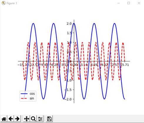
把下图做一些调整，要求：

1. 出现5个完整的波峰

2. 调大cos波形的幅度

3. 调大sin波形的频率

（2）作业分析及代码实现

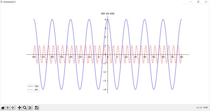
1. 5个完整波峰：这一点其实有点不懂，原图貌似已经出现了5个完整波峰了，姑且理解为需要5个完整波谷叭（可能我理解有问题叭），扩大x轴范围，生成数据时的x范围也扩大，考虑下面两点再设计具体实现；

2. 调大cos波形的幅度：在计算函数值时，用更大倍数乘以np.cos(x)即可，原图的是2，那么我调成4吧；

3. 调大sin波形的频率：众所周知，频率=ω/2π，所以只需调大ω即可，换言之，调大np.cos(kx)的k即可，原图k是2，同样我设成4；

4. 综上三点，可得核心代码：

x = np.linspace(-8 * np.pi, 8 * np.pi, 2048) # 生成从-8Π到8Π的2048个数据

cos, sin = 4 * np.cos(x), np.sin(4 * x)

5. 为使x坐标轴显示更加主流的π，我使用到函数set_xticklabels()：

xlabel = [str(i) + 'π' for i in range(-8, 9)]
xlabel = ['0' if i == '0π' else i for i in xlabel]
xlabel = ['π' if i == '1π' else i for i in xlabel]
xlabel = ['-π' if i == '-1π' else i for i in xlabel]
ax.set_xticklabels(xlabel)

6. 为画出坐标轴的十字形，需要使用到spines的隐藏功能和set_ticks_position()的设置边框位置功能：

# 画出十字形的坐标轴
ax.spines['right'].set_visible(False)               # 隐藏右边框
ax.spines['top'].set_visible(False)                 # 隐藏上边框
ax.spines['bottom'].set_position(('data', 0))       # 设置下边框到y轴0的位置
ax.xaxis.set_ticks_position('bottom')               # 刻度值设在下方
ax.spines['left'].set_position(('data', 0))         # 设置左边框到x轴0的位置
ax.yaxis.set_ticks_position('left')                 # 刻度值设在左侧

7. 综合上述分析，可编写程序如下：

"""绘制线图3"""
import csv
import numpy as np
import matplotlib.pyplot as plt
from matplotlib.pyplot import MultipleLocator
import pandas as pd
from random import randint

fig = plt.figure(figsize=(10, 10))          # 窗口大小
fig.canvas.set_window_title('Homework 4')   # 窗口标题
ax = plt.axes()                             # 创建坐标对象
ax.set_title("sin vs cos")                  # 线图标题

x = np.linspace(-8 * np.pi, 8 * np.pi, 2048)     # 生成从-8Π到8Π的2048个数据
# 分别计算cos和sin函数值：调大4倍cos函数的振幅，调大2倍sin函数的频率
cos, sin = 4 * np.cos(x), np.sin(4 * x)
ax.set_xticks([i * np.pi for i in range(-8, 9)])     # 设置x轴刻度，从-8Π到8Π
xlabel = [str(i) + 'π' for i in range(-8, 9)]
xlabel = ['0' if i == '0π' else i for i in xlabel]
xlabel = ['π' if i == '1π' else i for i in xlabel]
xlabel = ['-π' if i == '-1π' else i for i in xlabel]
ax.set_xticklabels(xlabel)
# cos曲线，颜色为蓝色，线宽为2，连续线
plt.plot(x, cos, color = 'blue', linewidth = 2, alpha = 0.5, linestyle = '-', label = 'cos')
# sin曲线，颜色为红色，线宽为2，间断线
plt.plot(x, sin, color = 'red', linewidth = 2, alpha = 0.5, linestyle = '--', label = 'sin')

# 画出十字形的坐标轴
ax.spines['right'].set_visible(False)               # 隐藏右边框
ax.spines['top'].set_visible(False)                 # 隐藏上边框
ax.spines['bottom'].set_position(('data', 0))       # 设置下边框到y轴0的位置
ax.xaxis.set_ticks_position('bottom')               # 刻度值设在下方
ax.spines['left'].set_position(('data', 0))         # 设置左边框到x轴0的位置
ax.yaxis.set_ticks_position('left')                 # 刻度值设在左侧

ax.legend(['cos', 'sin'], loc = 'lower left')       # 在左下角显示图例
plt.show()

（3）效果演示

2、作业五

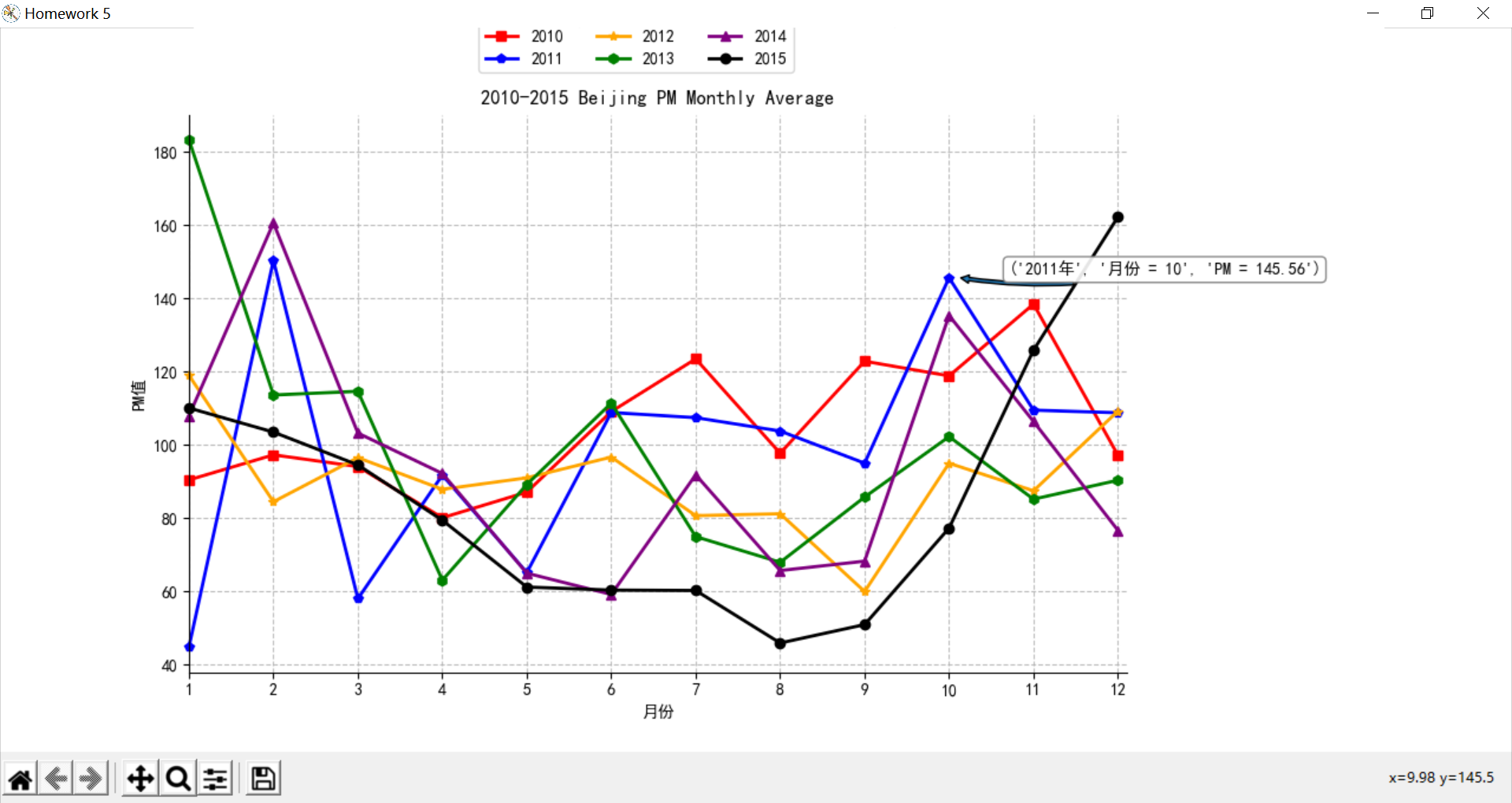
最后是重头戏，作业五。比较麻烦，需要综合前面所学的numpy和pandas来绘制线图，我为了让整幅图演示效果好一点也做了一些小小的工作。

（1）作业要求

用线图展示北京空气质量数据：

• 展示10-15年PM指数月平均数据的变化情况，一幅图中有6条曲线，每年1条曲线

（2）作业分析与代码实现

1. 对数据的处理：清洗空数据、计算平均值、取出各年份PM指数的月平均值，之前的作业有过类似的要求：

• 为了获得各年份PM指数的月平均值，我们首先求三个地方PM总数，另成一列PMsum；

• 同时因为有些格子是空的，所以要对每行参与计算PMsum的PM_Dongsi、PM_Dongsihuan、PM_Nongzhanguan、PM_US Post计算个数，另成一列PMcount；

• 最后用PMsum / PMcount即可得到每行的平均值，另成一列PMave；

• 取出各年份PM指数的月平均值，则对新的Dataframe使用group(['year', 'month']).mean()，此时PMave一行便转换成了各年份PM指数的月平均值；

• 将每年每月的PMave添加到列表PMave中，用于后续绘图

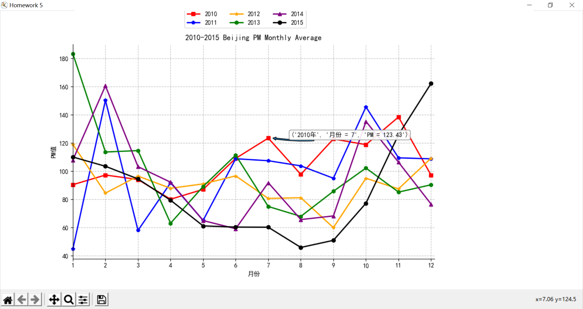
2. 搞定数据，绘图便变得简单起来，横坐标为month，纵坐标为PMave[i]（i代表年份，0对应2010），对每年的数据绘图。注意每年的数据点都要用不一样的点和颜色，比如2010年的是正方点、红色，示例语句如下：

# 2010：绘制颜色为红色、宽度为1像素的连续直线，数据点为正方点
plt.plot(month, PMave[0], 's', color = 'red', linewidth = 2.0, linestyle = '-', label = 'line1', clip_on=False)

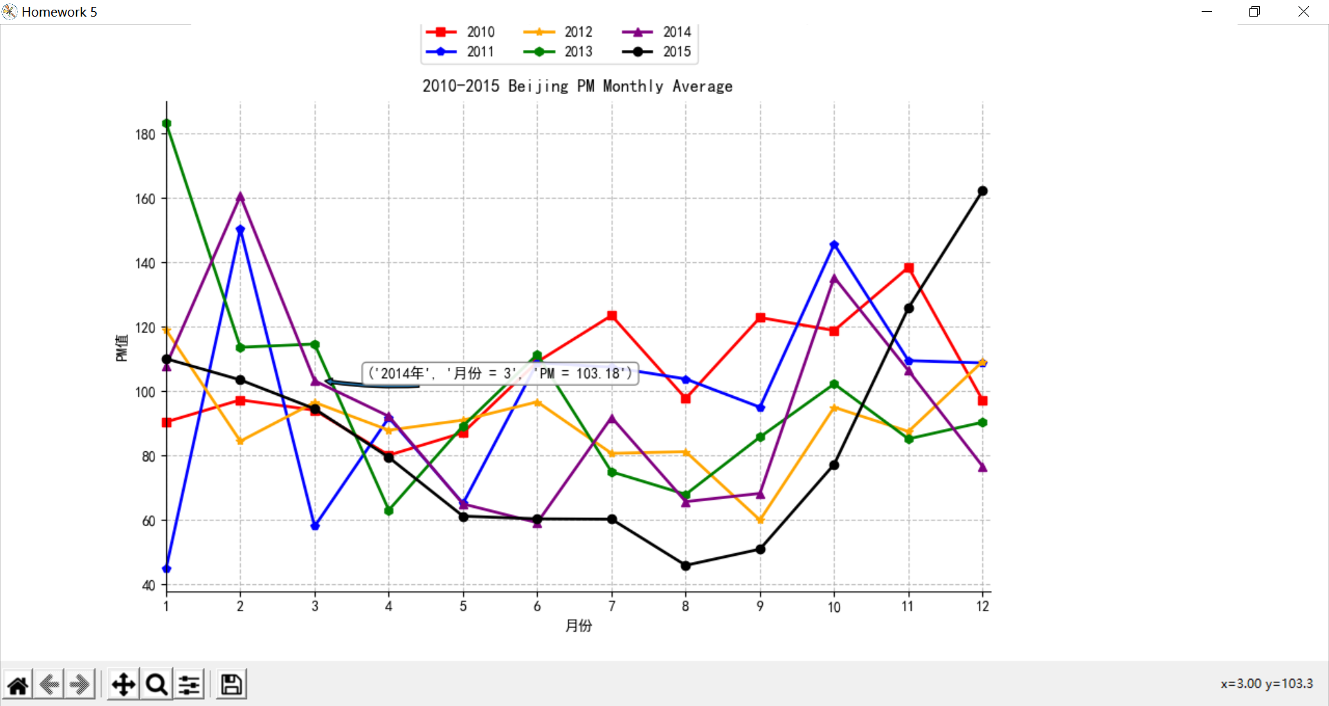
3. 接下来就是我为了使线图变得更加有效果做的工作。因为单单是线图没有显示数据标签的话，要对数据进一步了解就比较麻烦，但是如果直接把数据标签放在图上又会显得非常拥挤（毕竟有6条曲线），所以我想实现当鼠标移动到一个点上时，自动显示出该点的年份、月份和PM值。进一步查看PPT后，找到了我需要的函数，没错就是ax.annotate()；不过只是添加注释是没有用的，我需要在鼠标移动到点上再显示注释，进一步查找资料，bingo，就是set_visible()；所以我可以把每个点的注释先存入一个列表po_annotation，并在一开始全部设置为不可见set_visible(False)，等待鼠标移动到点上面，再设置成可见。

4. 构造函数on_move(event)，设置事件，当鼠标移动到点上时，显示po_annotation的内容。

5. 到现在就可以正式着手编写代码了，完整程序如下：

"""绘制线图4：用线图展示北京空气质量数据"""

import csv
import numpy as np
import matplotlib.pyplot as plt
from matplotlib.pyplot import MultipleLocator
import pandas as pd

# 读取文件
filename = 'BeijingPM20100101_20151231.csv'
df = pd.read_csv(filename, encoding = 'utf-8')

# 删除有空PM值的行
df.dropna(axis=0, how='all', subset=['PM_Dongsi','PM_Dongsihuan','PM_Nongzhanguan', 'PM_US Post'], inplace=True)

# 计算PM平均值
df['PMsum'] = df[['PM_Dongsi','PM_Dongsihuan','PM_Nongzhanguan', 'PM_US Post']].sum(axis=1)
df['PMcount'] = df[['PM_Dongsi','PM_Dongsihuan','PM_Nongzhanguan', 'PM_US Post']].count(axis=1)
df['PMave'] = round(df['PMsum'] / df['PMcount'],2)

# 取出各年份PM指数月平均数据
month = [i for i in range(1, 13)]
PMave = []
for i in range(2010, 2016):
    # 取出第i年的数据，对月求平均值
    aveM_df = df[df.year == i]
    aveM_df = aveM_df.groupby(['year', 'month']).mean()
    PMave.append(aveM_df.PMave)


fig = plt.figure(figsize=(10, 10))              # 窗口大小
fig.canvas.set_window_title('Homework 5')       # 窗口标题
ax = plt.axes()                                 # 创建坐标对象
ax.set_ylabel('PM值')
ax.set_xlabel('月份')
ax.set_title("2010-2015 Beijing PM Monthly Average") # 线图标题
ax.set_xticks([i for i in range(1, 13)])
plt.rcParams['font.sans-serif'] = ['SimHei']        # 添加对中文字体的支持

# 2010：绘制颜色为红色、宽度为1像素的连续直线，数据点为正方点
plt.plot(month, PMave[0], 's', color = 'red', linewidth = 2.0, linestyle = '-', label = 'line1', clip_on=False)
# 2011：绘制颜色为蓝色、宽度为1像素的连续直线，数据点为五角点
plt.plot(month, PMave[1], 'p', color = 'blue', linewidth = 2.0, linestyle = '-', label = 'line2', clip_on=False)
# 2012：绘制颜色为黄色、宽度为1像素的连续直线，数据点为星形点
plt.plot(month, PMave[2], '*', color = 'orange', linewidth = 2.0, linestyle = '-', label = 'line3', clip_on=False)
# 2013：绘制颜色为绿色、宽度为1像素的连续直线，数据点六边形1
plt.plot(month, PMave[3], 'h', color = 'green', linewidth = 2.0, linestyle = '-', label = 'line4', clip_on=False)
# 2014：绘制颜色为紫色、宽度为1像素的连续直线，数据点上三角
plt.plot(month, PMave[4], '^', color = 'purple', linewidth = 2.0, linestyle = '-', label = 'line5', clip_on=False)
# 2015：绘制颜色为黑色、宽度为1像素的连续直线，数据点圆点
plt.plot(month, PMave[5], 'bo', color = 'black', linewidth = 2.0, linestyle = '-', label = 'line6', clip_on=False)

""" 设置鼠标移动到点上时，显示点坐标（月份，PM）"""
po_annotation = []
for i in range(6):
    for j in range(1, 13):
        x = j                                   # 横坐标为月份
        y = round(PMave[i][2010 + i][j], 2)     # 纵坐标为PM
        print(x, y)
        point, = plt.plot(x, y)
        annotation = plt.annotate((str(2010 + i) + '年', '月份 = ' + str(x), 'PM = ' + str(y)), xy = (x + 0.1, y + 0.1), 
                                  xycoords = 'data', xytext = (x + 0.7, y + 0.7), textcoords = 'data', 
                                  horizontalalignment = "left", 
                                  arrowprops = dict(arrowstyle = "simple", connectionstyle = "arc3, rad = -0.1"), 
                                  bbox = dict(boxstyle = "round", facecolor = "w", edgecolor = "0.5", alpha = 0.9))
        annotation.set_visible(False)
        po_annotation.append([point, annotation])

def on_move(event):
    """设置事件，当鼠标移动到点上时，显示po_annotation的内容"""
    visibility_changed = False
    for point, annotation in po_annotation:
        should_be_visible = (point.contains(event)[0] == True)
        # print(point.contains(event)[0])
        if should_be_visible != annotation.get_visible():
            visibility_changed = True
            annotation.set_visible(should_be_visible)
    if visibility_changed:
        plt.draw()


plt.xlim(1, 12.1)    # 设置横轴的月份
ax.spines['right'].set_visible(False)               # 隐藏右边框
ax.spines['top'].set_visible(False)                 # 隐藏上边框
# 设置图例legend位置
box = ax.get_position()
ax.set_position([box.x0, box.y0, box.width * 0.8, box.height])     # 将图例放上面就box.height*0.8，放右边就box.width*0.8
ax.legend(['2010', '2011', '2012', '2013', '2014', '2015'], loc='center left', bbox_to_anchor = (0.3, 1.12), ncol = 3)
plt.grid(True, linestyle = '--', alpha = 0.8)       # 设置网格线

on_move_id = fig.canvas.mpl_connect('motion_notify_event', on_move)
plt.show()

6. 编写代码过程中，遇到一个问题，一开始我想对PMave[i]直接获取其中的数据时，发现无法直接用下标索引获取；我想到可能它的类型不是列表，于是打印PMave[i]的类型：

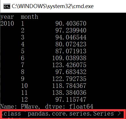
7. 这个类型没见过啊，于是上百度搜索，终于找到了这种数据类型的访问方法：

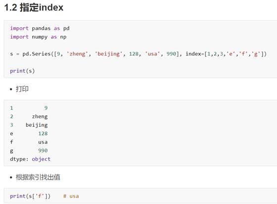
原来要访问该类型Series的元素，索引得是具体值，而不是下标。考虑下图打印内容，PMave要访问元素，需要两次索引：[year][month]；

最后终于用下面的访问方式解决了问题，开心！

for i in range(6):

for j in range(1, 13):

x = j # 横坐标为月份

y = round(PMave[i][2010 + i][j], 2) # 纵坐标为PM

（3）演示效果