pandas快速手册
修改列名
jdata_action2.rename(columns={'user_id':'heji'},inplace=True) #修改列名 将'user_id' 改为 'heji'
分组语句出图
jdata_action[['user_id','time_date']].groupby(['time_date']).count().plot.bar(figsize=(25,8))
滑窗计算
jdata_action2['roll']=jdata_action2.rolling(3, min_periods=1).mean()
转化时间函数 并按日期分组
jdata_action_date=jdata_action.groupby(pd.to_datetime(jdata_action['action_time']).dt.date)['user_id'].count()
根据所选内容出图
jdata_action2['roll'].plot.bar(figsize=(16,14))
查看dataframe信息
df.info()
删除某列信息
del df['abc']
去除重复的行信息
- 去除完全重复的行数据
data.drop_duplicates(inplace=True)
- 去除某几列重复的行数据
data.drop_duplicates(subset=['A','B'],keep='first',inplace=True)
subset: 列名,可选,默认为None
keep: {‘first’, ‘last’, False}, 默认值 ‘first’
first: 保留第一次出现的重复行,删除后面的重复行。
last: 删除重复项,除了最后一次出现。
False: 删除所有重复项。
删除某种条件的数据
jdata_action = jdata_action[-jdata_action['type'].isin([3,4])]
按照条件检索df
jdata_shop[jdata_shop['vender_id']==3666]
按照某字段分组,查看各组数据情况,并出图
jdata_action[['user_id','type']].groupby(['type']).count().plot.bar()
把某列转换为时间格式
jdata_action['time0']= pd.to_datetime(jdata_action['action_time'])
提取其中的日期
jdata_action['time_date']=jdata_action['time0'].dt.date
提起其中的时间
jdata_action['time_time']=jdata_action['time0'].dt.time
合并两个表
jdata_product=pd.merge(jdata_product,jdata_comment[['sku_id','comments']].groupby(['sku_id']).sum(),on='sku_id',how='left')
将df内容排序
jdata_shop[['vender_id','shop_id']].groupby(['vender_id']).count().sort_values(by='shop_id', ascending=False)
import xgboost as xgb
from sklearn.metrics import accuracy_score
import pandas as pd
import matplotlib.pyplot as plt
import numpy as np
pima = pd.read_csv("D:\\xgbtest\\pima-indians-diabetes.csv")
#取某列
pima['Outcome']
0 1
1 0
2 1
3 0
4 1
..
763 0
764 0
765 0
766 1
767 0
Name: Outcome, Length: 768, dtype: int64
#取某行
pima.iloc[0]
Pregnancies 6.000
Glucose 148.000
BloodPressure 72.000
SkinThickness 35.000
Insulin 0.000
BMI 33.600
DiabetesPedigreeFunction 0.627
Age 50.000
Outcome 1.000
Name: 0, dtype: float64
#x选出多个列
pima.loc[:,['Pregnancies','Glucose','BMI']]
| Pregnancies | Glucose | BMI | |
|---|---|---|---|
| 0 | 6 | 148 | 33.6 |
| 1 | 1 | 85 | 26.6 |
| 2 | 8 | 183 | 23.3 |
| 3 | 1 | 89 | 28.1 |
| 4 | 0 | 137 | 43.1 |
| ... | ... | ... | ... |
| 763 | 10 | 101 | 32.9 |
| 764 | 2 | 122 | 36.8 |
| 765 | 5 | 121 | 26.2 |
| 766 | 1 | 126 | 30.1 |
| 767 | 1 | 93 | 30.4 |
768 rows × 3 columns
#某个位置的值,纯整数索引
pima.iloc[[0],[0]]
| Pregnancies | |
|---|---|
| 0 | 6 |
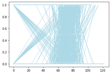
fig=plt.figure()
ax=fig.add_subplot(111)
x=pima['BloodPressure']
y=pima['Outcome']
ax.plot(x,y,color='lightblue',linewidth=1)
plt.show()
#查看部分data
pima.head()
| Pregnancies | Glucose | BloodPressure | SkinThickness | Insulin | BMI | DiabetesPedigreeFunction | Age | Outcome | |
|---|---|---|---|---|---|---|---|---|---|
| 0 | 6 | 148 | 72 | 35 | 0 | 33.6 | 0.627 | 50 | 1 |
| 1 | 1 | 85 | 66 | 29 | 0 | 26.6 | 0.351 | 31 | 0 |
| 2 | 8 | 183 | 64 | 0 | 0 | 23.3 | 0.672 | 32 | 1 |
| 3 | 1 | 89 | 66 | 23 | 94 | 28.1 | 0.167 | 21 | 0 |
| 4 | 0 | 137 | 40 | 35 | 168 | 43.1 | 2.288 | 33 | 1 |
# 对于非数字类型的数据(字符型 数据),可以使用pima.['这里填带统计的标签'].value_counts()统计分类数目
# 可以得到统计数目,得到平均数、方差等特征(当然是针对数字类型的数据)
pima.describe()
| Pregnancies | Glucose | BloodPressure | SkinThickness | Insulin | BMI | DiabetesPedigreeFunction | Age | Outcome | |
|---|---|---|---|---|---|---|---|---|---|
| count | 768.000000 | 768.000000 | 768.000000 | 768.000000 | 768.000000 | 768.000000 | 768.000000 | 768.000000 | 768.000000 |
| mean | 3.845052 | 120.894531 | 69.105469 | 20.536458 | 79.799479 | 31.992578 | 0.471876 | 33.240885 | 0.348958 |
| std | 3.369578 | 31.972618 | 19.355807 | 15.952218 | 115.244002 | 7.884160 | 0.331329 | 11.760232 | 0.476951 |
| min | 0.000000 | 0.000000 | 0.000000 | 0.000000 | 0.000000 | 0.000000 | 0.078000 | 21.000000 | 0.000000 |
| 25% | 1.000000 | 99.000000 | 62.000000 | 0.000000 | 0.000000 | 27.300000 | 0.243750 | 24.000000 | 0.000000 |
| 50% | 3.000000 | 117.000000 | 72.000000 | 23.000000 | 30.500000 | 32.000000 | 0.372500 | 29.000000 | 0.000000 |
| 75% | 6.000000 | 140.250000 | 80.000000 | 32.000000 | 127.250000 | 36.600000 | 0.626250 | 41.000000 | 1.000000 |
| max | 17.000000 | 199.000000 | 122.000000 | 99.000000 | 846.000000 | 67.100000 | 2.420000 | 81.000000 | 1.000000 |
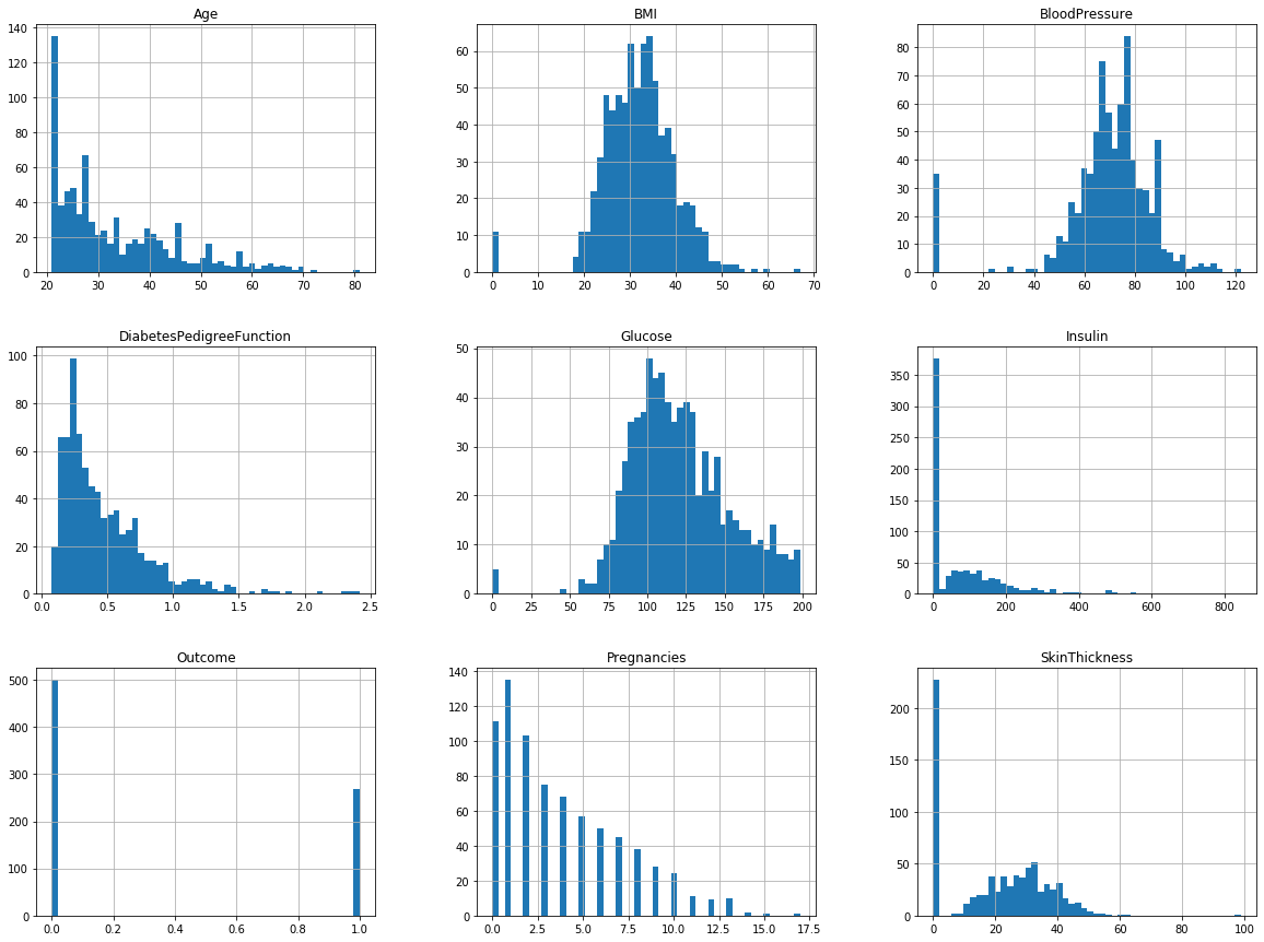
# 可以显示该标签下的数据分布,50表示y轴的间隔,以直方图显示,横轴表示数值范围,y轴表示数量
# bins指bin(箱子)的个数,即每张图柱子的个数
# figsize指每张图的尺寸大小

pima.hist(bins=50,figsize=(20,15))
array([[<matplotlib.axes._subplots.AxesSubplot object at 0x0000010F597CC988>,
<matplotlib.axes._subplots.AxesSubplot object at 0x0000010F59690348>,
<matplotlib.axes._subplots.AxesSubplot object at 0x0000010F5987B7C8>],
[<matplotlib.axes._subplots.AxesSubplot object at 0x0000010F59053208>,
<matplotlib.axes._subplots.AxesSubplot object at 0x0000010F59080BC8>,
<matplotlib.axes._subplots.AxesSubplot object at 0x0000010F590BA5C8>],
[<matplotlib.axes._subplots.AxesSubplot object at 0x0000010F590E8E48>,
<matplotlib.axes._subplots.AxesSubplot object at 0x0000010F59113F88>,
<matplotlib.axes._subplots.AxesSubplot object at 0x0000010F5911EB88>]],
dtype=object)
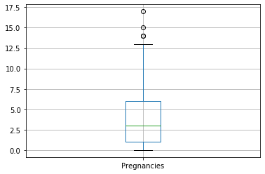
# 可以显示该标签下的数值分布,观察分布是否均衡 箱形图或盒图
pima.boxplot(column='Pregnancies')
<matplotlib.axes._subplots.AxesSubplot at 0x10f5a32b888>
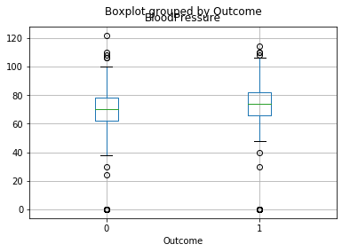
# 可以将标签1下的数据再按照标签2进行数值分布绘制
pima.boxplot(column='BloodPressure', by = 'Outcome')
<matplotlib.axes._subplots.AxesSubplot at 0x10f5a9660c8>
#查看两列相关性
pima['BloodPressure'].corr(pima['Age'])
0.23952794642136363
#查看两列相关性
pima.corr()
| Pregnancies | Glucose | BloodPressure | SkinThickness | Insulin | BMI | DiabetesPedigreeFunction | Age | Outcome | |
|---|---|---|---|---|---|---|---|---|---|
| Pregnancies | 1.000000 | 0.129459 | 0.141282 | -0.081672 | -0.073535 | 0.017683 | -0.033523 | 0.544341 | 0.221898 |
| Glucose | 0.129459 | 1.000000 | 0.152590 | 0.057328 | 0.331357 | 0.221071 | 0.137337 | 0.263514 | 0.466581 |
| BloodPressure | 0.141282 | 0.152590 | 1.000000 | 0.207371 | 0.088933 | 0.281805 | 0.041265 | 0.239528 | 0.065068 |
| SkinThickness | -0.081672 | 0.057328 | 0.207371 | 1.000000 | 0.436783 | 0.392573 | 0.183928 | -0.113970 | 0.074752 |
| Insulin | -0.073535 | 0.331357 | 0.088933 | 0.436783 | 1.000000 | 0.197859 | 0.185071 | -0.042163 | 0.130548 |
| BMI | 0.017683 | 0.221071 | 0.281805 | 0.392573 | 0.197859 | 1.000000 | 0.140647 | 0.036242 | 0.292695 |
| DiabetesPedigreeFunction | -0.033523 | 0.137337 | 0.041265 | 0.183928 | 0.185071 | 0.140647 | 1.000000 | 0.033561 | 0.173844 |
| Age | 0.544341 | 0.263514 | 0.239528 | -0.113970 | -0.042163 | 0.036242 | 0.033561 | 1.000000 | 0.238356 |
| Outcome | 0.221898 | 0.466581 | 0.065068 | 0.074752 | 0.130548 | 0.292695 | 0.173844 | 0.238356 | 1.000000 |
#生成排名
pima['Pregnancies'].rank()
0 574.5
1 179.0
2 663.5
3 179.0
4 56.0
...
763 722.5
764 298.0
765 521.0
766 179.0
767 179.0
Name: Pregnancies, Length: 768, dtype: float64
# rolling()遍历的是移动窗口的数据 由于窗口大小为3(window),前两个元素有空值,第三个元素的值将是n,n-1和n-2元素的平均值。  下例中 取得均值
pima['Pregnancies'].rolling(window=3).mean()
0 NaN
1 NaN
2 5.000000
3 3.333333
4 3.000000
...
763 9.333333
764 7.000000
765 5.666667
766 2.666667
767 2.333333
Name: Pregnancies, Length: 768, dtype: float64
# 数据补全
df = pd.DataFrame(np.random.randn(5, 3), index=['a', 'c', 'e', 'f','h'],columns=['one', 'two', 'three'])
df = df.reindex(['a', 'b', 'c', 'd', 'e', 'f', 'g', 'h'])

print (df)
print (df['one'].fillna(df['one'].median()))  #用中位数填充缺失值
one two three
a 0.018628 -0.684334 1.280671
b NaN NaN NaN
c 1.043673 -1.065631 -0.107962
d NaN NaN NaN
e 0.321906 1.229281 -0.599733
f 0.094914 -2.588472 -0.032368
g NaN NaN NaN
h 1.349480 -0.996243 1.670260
a 0.018628
b 0.321906
c 1.043673
d 0.321906
e 0.321906
f 0.094914
g 0.321906
h 1.349480
Name: one, dtype: float64
df = pd.DataFrame({'one':[10,20,30,40,50,2000],'two':[1000,0,30,40,50,60]})
#替换 用10 换1000;60换2000.可以同时替换多个值
print (df.replace({1000:10,2000:60}))
one two
0 10 10
1 20 0
2 30 30
3 40 40
4 50 50
5 60 60
ipl_data = {'Team': ['Riders', 'Riders', 'Devils', 'Devils', 'Kings','kings', 'Kings', 'Kings', 'Riders', 'Royals', 'Royals', 'Riders'],
         'Rank': [1, 2, 2, 3, 3,4 ,1 ,1,2 , 4,1,2],
         'Year': [2014,2015,2014,2015,2014,2015,2016,2017,2016,2014,2015,2017],
         'Points':[876,789,863,673,741,812,756,788,694,701,804,690]}
df = pd.DataFrame(ipl_data)
#按'Team'分组,并打印结果
print (df.groupby('Team').groups)
{'Devils': Int64Index([2, 3], dtype='int64'), 'Kings': Int64Index([4, 6, 7], dtype='int64'), 'Riders': Int64Index([0, 1, 8, 11], dtype='int64'), 'Royals': Int64Index([9, 10], dtype='int64'), 'kings': Int64Index([5], dtype='int64')}
#按'Year'分组,并迭代输出
grouped = df.groupby('Year')
for name,group in grouped:
    print (name)
    print (group)
2014
Team Rank Year Points
0 Riders 1 2014 876
2 Devils 2 2014 863
4 Kings 3 2014 741
9 Royals 4 2014 701
2015
Team Rank Year Points
1 Riders 2 2015 789
3 Devils 3 2015 673
5 kings 4 2015 812
10 Royals 1 2015 804
2016
Team Rank Year Points
6 Kings 1 2016 756
8 Riders 2 2016 694
2017
Team Rank Year Points
7 Kings 1 2017 788
11 Riders 2 2017 690
# 使用get_group()方法,可以选择一个组。
print (grouped.get_group(2014))
Team Rank Year Points
0 Riders 1 2014 876
2 Devils 2 2014 863
4 Kings 3 2014 741
9 Royals 4 2014 701
# 聚合函数为每个组返回单个聚合值
grouped = df.groupby('Year')
print (grouped['Points'].agg(np.mean))
Year
2014 795.25
2015 769.50
2016 725.00
2017 739.00
Name: Points, dtype: float64
# 查看每个分组的大小的方法
grouped = df.groupby('Team')
print (grouped.agg(np.size))
Rank Year Points
Team
Devils 2 2 2
Kings 3 3 3
Riders 4 4 4
Royals 2 2 2
kings 1 1 1
# 通过分组系列,还可以传递函数的列表或字典来进行聚合
grouped = df.groupby('Team')
agg = grouped['Points'].agg([np.sum, np.mean, np.std])
print (agg)
sum mean std
Team
Devils 1536 768.000000 134.350288
Kings 2285 761.666667 24.006943
Riders 3049 762.250000 88.567771
Royals 1505 752.500000 72.831998
kings 812 812.000000 NaN
# 过滤根据定义的标准过滤数据并返回数据的子集
filter = df.groupby('Team').filter(lambda x: len(x) >= 3)
print (filter)
Team Rank Year Points
0 Riders 1 2014 876
1 Riders 2 2015 789
4 Kings 3 2014 741
6 Kings 1 2016 756
7 Kings 1 2017 788
8 Riders 2 2016 694
11 Riders 2 2017 690
# 类似SQL的两个表连接
left = pd.DataFrame({
         'id':[1,2,3,4,5],
         'Name': ['Alex', 'Amy', 'Allen', 'Alice', 'Ayoung'],
         'subject_id':['sub1','sub2','sub4','sub6','sub5']})
right = pd.DataFrame(
         {'id':[1,2,3,4,5],
         'Name': ['Billy', 'Brian', 'Bran', 'Bryce', 'Betty'],
         'subject_id':['sub2','sub4','sub3','sub6','sub5']})
rs = pd.merge(left,right,on='id')  #等值连接
print(rs)
id Name_x subject_id_x Name_y subject_id_y
0 1 Alex sub1 Billy sub2
1 2 Amy sub2 Brian sub4
2 3 Allen sub4 Bran sub3
3 4 Alice sub6 Bryce sub6
4 5 Ayoung sub5 Betty sub5
# 合并多个键上的两个数据框
rs = pd.merge(left,right,on=['id','subject_id'])
print(rs)
id Name_x subject_id Name_y
0 4 Alice sub6 Bryce
1 5 Ayoung sub5 Betty
#left 相当于 LEFT OUTER JOIN
# right 相当于 RIGHT OUTER JOIN
# outer 相当于 FULL OUTER JOIN
# inner 相当于INNER JOIN
rs = pd.merge(left, right, on='subject_id', how='left')
print (rs)
id_x Name_x subject_id id_y Name_y
0 1 Alex sub1 NaN NaN
1 2 Amy sub2 1.0 Billy
2 3 Allen sub4 2.0 Brian
3 4 Alice sub6 4.0 Bryce
4 5 Ayoung sub5 5.0 Betty
#生成时间
#取当前时间
print(pd.datetime.now())
2020-02-29 11:15:30.372039
# 创建一个时间戳
time = pd.Timestamp('2018-11-01')
print(time)
2018-11-01 00:00:00
# 转换成整数或浮动时期。这些的默认单位是纳秒(因为这些是如何存储时间戳的)。
time = pd.Timestamp(1588686880,unit='s')
print(time)
2020-05-05 13:54:40
# 创建一个时间范围
time = pd.date_range("12:00", "23:59", freq="30min").time
print(time)
[datetime.time(12, 0) datetime.time(12, 30) datetime.time(13, 0)
datetime.time(13, 30) datetime.time(14, 0) datetime.time(14, 30)
datetime.time(15, 0) datetime.time(15, 30) datetime.time(16, 0)
datetime.time(16, 30) datetime.time(17, 0) datetime.time(17, 30)
datetime.time(18, 0) datetime.time(18, 30) datetime.time(19, 0)
datetime.time(19, 30) datetime.time(20, 0) datetime.time(20, 30)
datetime.time(21, 0) datetime.time(21, 30) datetime.time(22, 0)
datetime.time(22, 30) datetime.time(23, 0) datetime.time(23, 30)]
# 改变时间的频率
time = pd.date_range("12:00", "23:59", freq="H").time
print(time)
[datetime.time(12, 0) datetime.time(13, 0) datetime.time(14, 0)
datetime.time(15, 0) datetime.time(16, 0) datetime.time(17, 0)
datetime.time(18, 0) datetime.time(19, 0) datetime.time(20, 0)
datetime.time(21, 0) datetime.time(22, 0) datetime.time(23, 0)]
# 要转换类似日期的对象
time = pd.to_datetime(pd.Series(['Jul 31, 2009','2019-10-10','2019/1/2','20190101', None]))
print(time)
0 2009-07-31
1 2019-10-10
2 2019-01-02
3 2019-01-01
4 NaT
dtype: datetime64[ns]
# 创建一个日期范围通过指定周期和频率,使用date.range()函数就可以创建日期序列。 默认情况下,范围的频率是天。
datelist = pd.date_range('2020/11/21', periods=5)
print(datelist)
DatetimeIndex(['2020-11-21', '2020-11-22', '2020-11-23', '2020-11-24',
'2020-11-25'],
dtype='datetime64[ns]', freq='D')
# 更改日期频率
datelist = pd.date_range('2020/11/21', periods=5,freq='M')
print(datelist)
DatetimeIndex(['2020-11-30', '2020-12-31', '2021-01-31', '2021-02-28',
'2021-03-31'],
dtype='datetime64[ns]', freq='M')
# bdate_range()用来表示商业日期范围,不同于date_range(),它不包括星期六和星期天。观察到11月3日以后,日期跳至11月6日,不包括4日和5日(因为它们是周六和周日)。
datelist = pd.date_range('2011/11/03', periods=5)
print(datelist)
DatetimeIndex(['2011-11-03', '2011-11-04', '2011-11-05', '2011-11-06',
'2011-11-07'],
dtype='datetime64[ns]', freq='D')
#时间范围
start = pd.datetime(2017, 11, 1)
end = pd.datetime(2017, 11, 5)
dates = pd.date_range(start, end)
print(dates)
DatetimeIndex(['2017-11-01', '2017-11-02', '2017-11-03', '2017-11-04',
'2017-11-05'],
dtype='datetime64[ns]', freq='D')
# 时间差(Timedelta)
timediff = pd.Timedelta('2 days 2 hours 15 minutes 30 seconds')
print(timediff)
2 days 02:15:30
timediff = pd.Timedelta(6,unit='h')
print(timediff)
0 days 06:00:00
timediff = pd.Timedelta(days=2)
print(timediff)
2 days 00:00:00
#构建两组数据
s = pd.Series(pd.date_range('2012-1-1', periods=3, freq='D'))
td = pd.Series([ pd.Timedelta(days=i) for i in range(3) ])
df = pd.DataFrame(dict(A = s, B = td))
print(df)
A B
0 2012-01-01 0 days
1 2012-01-02 1 days
2 2012-01-03 2 days
# 相加操作
df['C']=df['A']+df['B']
print(df)
A B C
0 2012-01-01 0 days 2012-01-01
1 2012-01-02 1 days 2012-01-03
2 2012-01-03 2 days 2012-01-05
# 相减操作
df['D']=df['C']-df['B']
print(df)
A B C D
0 2012-01-01 0 days 2012-01-01 2012-01-01
1 2012-01-02 1 days 2012-01-03 2012-01-02
2 2012-01-03 2 days 2012-01-05 2012-01-03
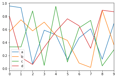
#基本绘图
df = pd.DataFrame(np.random.rand(10,4),columns=['a','b','c','d'])
df.plot()
<matplotlib.axes._subplots.AxesSubplot at 0x10f5dbe95c8>
# 条形图
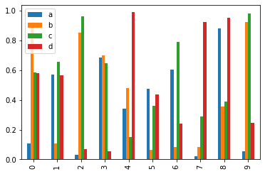
df = pd.DataFrame(np.random.rand(10,4),columns=['a','b','c','d'])
df.plot.bar()
<matplotlib.axes._subplots.AxesSubplot at 0x10f5dc624c8>
# 堆积条形图
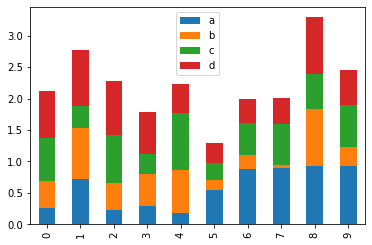
df = pd.DataFrame(np.random.rand(10,4),columns=['a','b','c','d'])
df.plot.bar(stacked=True)
<matplotlib.axes._subplots.AxesSubplot at 0x10f5de41e48>
# 水平条形图
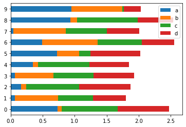
df = pd.DataFrame(np.random.rand(10,4),columns=['a','b','c','d'])
df.plot.barh(stacked=True)
<matplotlib.axes._subplots.AxesSubplot at 0x10f5df29d88>
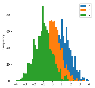
# 直方图
df = pd.DataFrame({'a':np.random.randn(1000)+1,'b':np.random.randn(1000),'c':np.random.randn(1000) - 1}, columns=['a', 'b', 'c'])
df.plot.hist(bins=50, figsize=(5,5))
# bins指bin(箱子)的个数,即每张图柱子的个数
# figsize指每张图的尺寸大小
<matplotlib.axes._subplots.AxesSubplot at 0x10f5f644248>
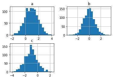
# 要为每列绘制不同的直方图
# df=pd.DataFrame({'a':np.random.randn(1000)+1,'b':np.random.randn(1000),'c':np.random.randn(1000) - 1}, columns=['a', 'b', 'c'])
df.hist(bins=20)
array([[<matplotlib.axes._subplots.AxesSubplot object at 0x0000010F5FACE7C8>,
<matplotlib.axes._subplots.AxesSubplot object at 0x0000010F5FACE5C8>],
[<matplotlib.axes._subplots.AxesSubplot object at 0x0000010F5FB3C108>,
<matplotlib.axes._subplots.AxesSubplot object at 0x0000010F5FB72AC8>]],
dtype=object)
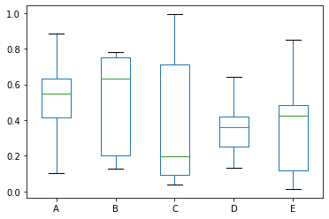
# 箱形图
# Boxplot可以绘制调用Series.box.plot()和DataFrame.box.plot()或DataFrame.boxplot()来可视化每列中值的分布。
df = pd.DataFrame(np.random.rand(10, 5), columns=['A', 'B', 'C', 'D', 'E'])
df.plot.box()
<matplotlib.axes._subplots.AxesSubplot at 0x10f5fbd2788>
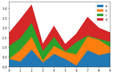
# 区域块图形 可以使用Series.plot.area()或DataFrame.plot.area()方法创建区域图形
df = pd.DataFrame(np.random.rand(10, 4), columns=['a', 'b', 'c', 'd'])
df.plot.area()
<matplotlib.axes._subplots.AxesSubplot at 0x10f5fd7f708>
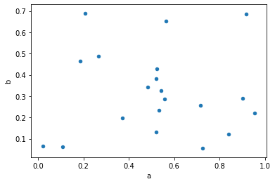
# 散点图形
df = pd.DataFrame(np.random.rand(20, 4), columns=['a', 'b', 'c', 'd'])
df.plot.scatter(x='a', y='b')
<matplotlib.axes._subplots.AxesSubplot at 0x10f611e0e08>
#折线图
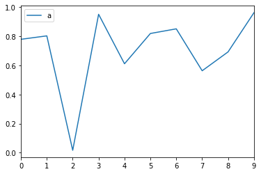
df = pd.DataFrame({'a':np.random.rand(10)})
df.plot(kind='line')
<matplotlib.axes._subplots.AxesSubplot at 0x10f6145f588>
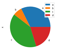
# 饼状图
df = pd.DataFrame(3 * np.random.rand(4), index=['a', 'b', 'c', 'd'], columns=['x'])
df.plot.pie(subplots=True)
array([<matplotlib.axes._subplots.AxesSubplot object at 0x0000010F6157B588>],
dtype=object)


 浙公网安备 33010602011771号