VAE LSTM shape
LSTM input and output shape:
- The input of the LSTM is always is a 3D array. (batch_size, time_steps, seq_len)
- The output of the LSTM could be a 2D array or 3D array depending upon the return_sequences argument.
- If return_sequence is False, the output is a 2D array. (batch_size, units)
- If return_sequence is True, the output is a 3D array. (batch_size, time_steps, units)
LSTM input and output shape of Pytorch:
PyTorch provides implementations for most of the commonly used entities from layers such as LSTMs, CNNs and GRUs to optimizers like SGD, Adam. The general paradigm to use any of these entities is to first create an instance of torch.nn.entity with some required parameters. As an example, here’s how we instantiate an lstm.
# Step 1
lstm = torch.nn.LSTM(input_size=5, hidden_size=10, batch_first=True)
Next, we call this object with the inputs as parameters when we actually want to run an LSTM over some inputs. This is shown in the third line below.
below.
lstm_in = torch.rand(40, 20, 5)
hidden_in = (torch.zeros(1, 40, 10), torch.zeros(1, 40, 10)) #(h0,c0)
# Step 2
lstm_out, lstm_hidden = lstm(lstm_in, hidden_in)
A note on dimensionality
During step 2 of the general paradigm, torch.nn.LSTM expects the input to be a 3D input tensor of size (seq_len, batch, embedding_dim), and returns an output tensor of the size (seq_len, batch, hidden_dim).
As an example, consider the input-output pair ('ERPDRF', 'SECRET'). Using an embedding_dim of 5, the 6 letter long input ERPDRF is transformed into an input tensor of size 6 x 1 x 5. If hidden_dim is 10, the input is processed by the LSTM into an output tensor of size 6 x 1 x 10.
Transform the outputs
The general workaround is to transform the D dimensional tensor into a V dimensional tensor through what is called an affine (or linear) transform. Sparing the definitions aside, the idea is to use matrix multiplication to get the desired dimensions.
Let’s say the LSTM produces an output tensor O of size seq_len x batch x hidden_dim. Recall that we only feed in one example at a time, so batch is always 1. This essentially gives us an output tensor O of size seq_len x hidden_dim. Now if we multiply this output tensor with another tensor W of size hidden_dim x embedding_dim, the resultant tensor R=O×W has a size of seq_len x embedding_dim. Isn’t this exactly what we wanted?
To implement the linear layer, … you guessed it! We create an instance of torch.nn.Linear. This time, the docs list the required parameters as in_features: size of each input sample and out_features: size of each output sample. Note that this only transforms the last dimension of the input tensor. So for example, if we pass in an input tensor of size (d1, d2, d3, ..., dn, in_features), the output tensor will have the same size for all but the last dimension, and will be a tensor of size (d1, d2, d3, ..., dn, out_features).
Encoder-Decoder model:
The model consists of 3 parts: encoder, intermediate (encoder) vector and decoder.
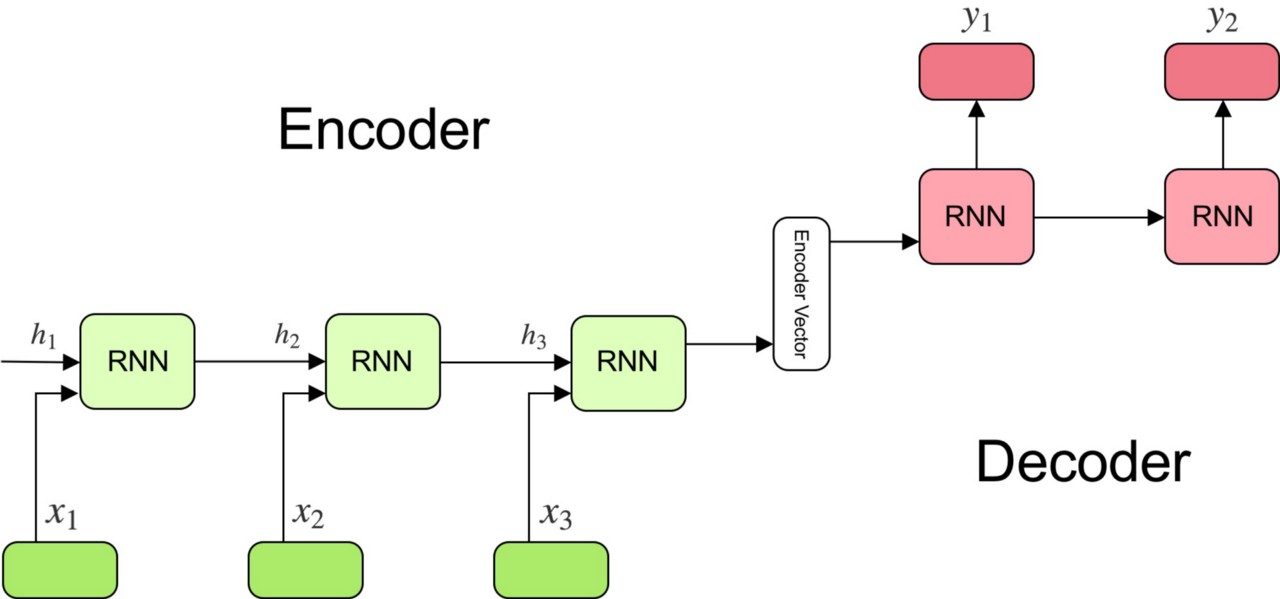
Encoder
- A stack of several recurrent units (LSTM or GRU cells for better performance) where each accepts a single element of the input sequence, collects information for that element and propagates it forward.
- In question-answering problem, the input sequence is a collection of all words from the question. Each word is represented as x_i where i is the order of that word.
- The hidden states h_i are computed using the formula:
This simple formula represents the result of an ordinary recurrent neural network. As you can see, we just apply the appropriate weights to the previous hidden state h_(t-1) and the input vector x_t.
Encoder Vector
- This is the final hidden state produced from the encoder part of the model. It is calculated using the formula above.
- This vector aims to encapsulate the information for all input elements in order to help the decoder make accurate predictions.
- It acts as the initial hidden state of the decoder part of the model.
Decoder
- A stack of several recurrent units where each predicts an output y_t at a time step t.
- Each recurrent unit accepts a hidden state from the previous unit and produces and output as well as its own hidden state.
- In the question-answering problem, the output sequence is a collection of all words from the answer. Each word is represented as y_i where i is the order of that word.
- Any hidden state h_i is computed using the formula:

As you can see, we are just using the previous hidden state to compute the next one.
- The output y_t at time step t is computed using the formula:
Shape connection between encoder and decoder:
There’s a problem though.
We must connect the encoder to the decoder, and they do not fit.
That is, the encoder will produce a 2-dimensional matrix of outputs, where the length is defined by the number of memory cells in the layer. The decoder is an LSTM layer that expects a 3D input of [samples, time steps, features] in order to produce a decoded sequence of some different length defined by the problem.
- One method: The RepeatVector layer can be used like an adapter to fit the encoder and decoder parts of the network together.
- the other method: a common method to implement seq2seq is to use the encoder’s output as the initial value for the decoder inner state. Each token the decoder outputs is then fed back as input to the decoder.
but which way is better, still need to be tested. however, the second method can be used for attention.
The output of the decoder:
The output of the decoder aims to model the distribution p(x|t), i.e. the distribution of data x given the latent variable t. Therefore, in principle, it should always be probabilistic.
However, in some cases, people simply use the mean squared error as the loss and, as you said, the output of the decoder is the actual predicted data points. Note that this approach can also be viewed as probabilistic, in the sense that it is is equivalent to modeling p(x|t) as Gaussian with identity covariance, p(x|t)=N(x|μ(t),I). In this case, the output of the decoder is the mean μ(t) and, therefore, for an example xi, you get the following reconstruction loss:
which, as you can see, is proportional to the mean squared error (plus some constant).
Question 2:
Bernoulli distribution makes sense for grey scale pixels.
This is not quite true. The correct statement would be that Bernoulli distribution makes sense for black and white (i.e. binary) images. The Bernoulli distribution is binary, so it assumes that observations may only have two possible outcomes. It is true that people sometimes use it for grayscale images, but this is an abusive interpretation of the VAE. It may work pretty well for datasets that are almost black and white, like MNIST. However, a binarized version of the MNIST dataset exists and, in rigor, this is the version that should be used together with a Bernoulli VAE.
But for something like stock returns, we would want some other distribution, such as a t-distribution. In this case, the output of the encoder would be 3 vectors, 1 for location, 1 for scale, and 1 for degrees of freedom, right?
I would try a Gaussian first, p(x|t)=N(x|μ(t),σ2(t)), so the decoder would output two values, μ(t)μ(t) and σ2(t)σ2(t). But yeah, if you really want a t-distribution, then that is the way to go.
Reference:
-
Building your first RNN with PyTorch 0.4
- Understanding LSTM input
- http://www.wildml.com/2016/01/attention-and-memory-in-deep-learning-and-nlp/

 浙公网安备 33010602011771号