
Realitymining 数据集简单介绍与使用
数据集的官网 http://realitycommons.media.mit.edu/index.html(可能需要FQ) ,下面是数据集的简要介绍(摘自官方网站)
The goal of this experiment was to explore the capabilities of the smart phones that enabled social scientists to investigate human interactions beyond the traditional survey based methodology or the traditional simulation base methodology. The subjects were 75 students or faculty in the MIT Media Laboratory, and 25 incoming students at the MIT Sloan business school adjacent to the Media Laboratory. Of the 75 Media Lab participants, 20 were incoming masters students and 5 were incoming MIT freshman, and the rest had remained in the Media Lab for at least a year.
本文的初衷是在尽可能保户用户隐私的情况下对用户进行好友推荐,而不是像许多文献那样(这里指获取用户的隐私数据,我个人觉得不可行.),这里只是在实验的情况下,因为在现实生活中,不会有人经常开着无线设备而为了得到一些无关紧要的推荐结果.本文思想是利用 bluetooth 数据,发现用户好友关系,对其简单的排序结果对用户进行好友推荐,并与随推荐结果相比较,验证其方法的可以行性.实验使用的数据集是 2004年,mit的数据,不知道有没近些年的相关数据集,有感兴趣的可以交流一下.
抽取部分自己需要的数据:
 1 %获取需要的数据,
 2 %转入原始数据
 3 data = load('realitymining.mat');
 4 %subject数据  struct 数组   1*106  struct
 5 %结构体数组  data.s(0)  - data.s(106)
 6 %可以采用这种方式 给新 结构数组 赋值   datalite.s(0).mac  =  data.s(0).mac
 7
 8 % 新建一个结构体数组,可采用 使用直接引用方式定义结构
 9 s = struct([]);
10 n = 1;
11 while (n~=107)
12     %添加想要的数据
13     s(n).mac = data.s(n).mac;
14     s(n).device_list_macs = data.s(n).device_list_macs;
15     s(n).device_list_names = data.s(n).device_list_names;
16     %这三列数据的 列数应该是相等的.
17     s(n).device_date = data.s(n).device_date;
18     s(n).device_names = data.s(n).device_names;
19     s(n).device_macs = data.s(n).device_macs;
20     s(n).neighborhood = data.s(n).neighborhood;
21     s(n).my_office = data.s(n).my_office;
22     n=n+1;
23
24 end
25
26 network = data.network;
27 save 'slite' 's' 'network'
根据好友关系绘制拓扑图,结点显示 bluetooth的 mac号.
function ND_netplot(network,s)
    A = network.friends;
    [n,m]=size(A);
    w=floor(sqrt(n));
    h=floor(n/w);
    x = zeros(1,w*h);
    y = zeros(1,w*h);
    index = 0;
    for i=1:h           %使产生的随机点有其范围,使显示分布的更广
        for j=1:w
            index = index +1;
            x(index)=10*rand(1)+(j-1)*10;
            y(index) =10*rand(1)+(i-1)*10;

        end
    end

    ed=n-h*w;
    for i=1:ed
       index = index +1;
       x(index)=10*rand(1)+(i-1)*10;
       y(index)=10*rand(1)+h*10;
    end
    plot(x,y,'ok');

    title('网络拓扑图');
    for i=1:n
        for j=1:n
            if A(i,j) == 1
                c=num2str(A(i,j));                      %将A中的权值转化为字符型
                text((x(i)+x(j))/2,(y(i)+y(j))/2,c,'Fontsize',10);  %显示边的权值
                if i ~= j
                    arrow([x(j),y(j)],[x(i),y(i)]);         %带箭头的连线
                end
            end
            %hold on;
        end
        if i< 94
            %这里不显示点的序号,显示  mac地址.
            sub_index = network.sub_sort(i);
            mac = ['--',num2str(s(sub_index).mac)];
            text(x(i),y(i),[num2str(sub_index),mac],'Fontsize',9,'color','r');   %显示点的序号
            disp([num2str(sub_index),mac]);
        end

    end
end
结果如图:
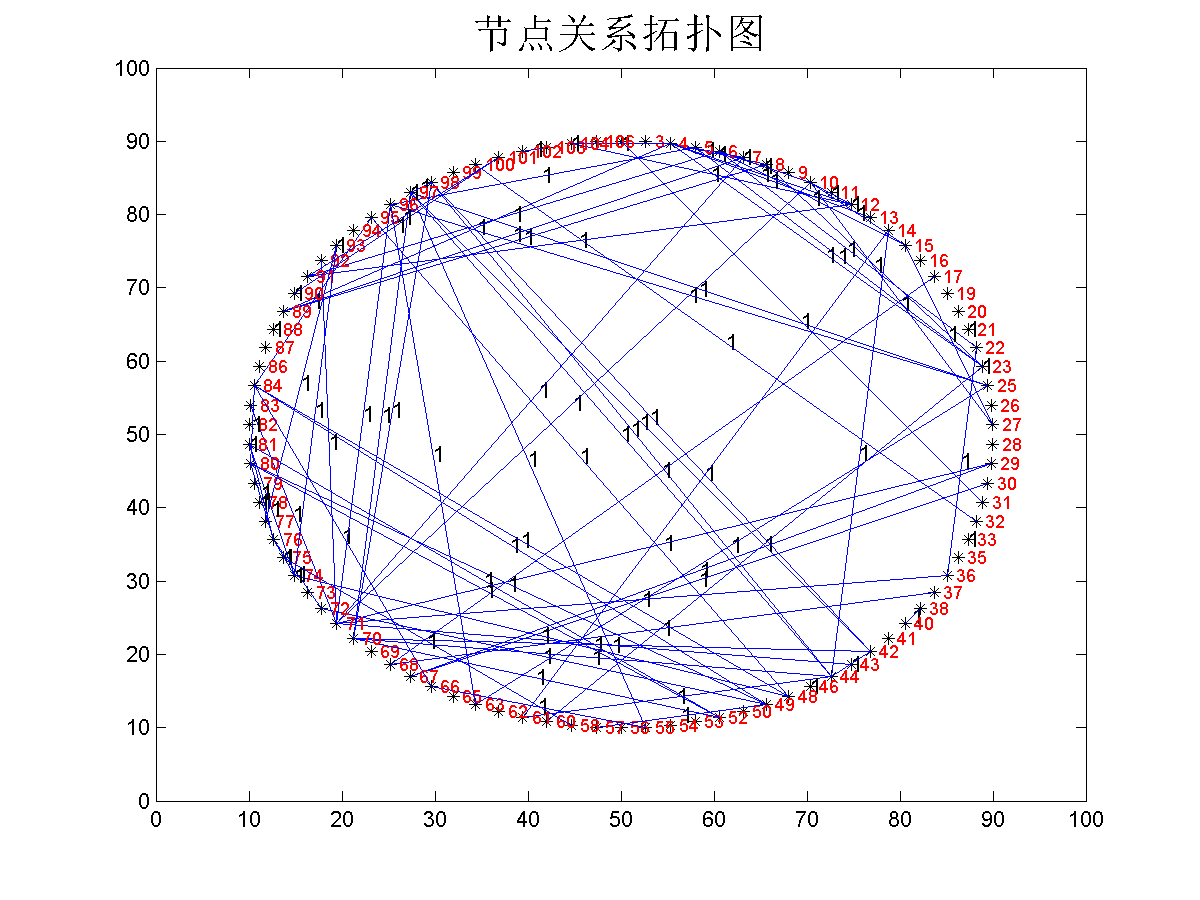
到这里并不没做什么实际性的工作,只是将需要的数据分离出现.并将好友关系,以有向图的方式绘制出来 .
用户 hash_number 与之对应的 bluetooth mac
3--61961024887
4--61961024891
5--61961024929
6--61961024956
7--61961024927
8--61961025059
9--61961078506
10--61961024943
11--61961024868
12--61961078565
13--61961024950
14--61961078566
15--61961024968
16--61961024963
17--61960619991
19--61961024937
20--61961024824
21--61961024912
22--61961024938
23--61961025033
25--61960946218
26--61961078573
27--61961024853
28--61961078595
29--61960946349
30--61960946207
31--61961078619
32--61961024881
33--61961025202
35--61961024951
36--61961025054
37--61961024911
38--61961025073
40--61961078559
41--61965359991
42--61965359983
43--61965360050
44--61965359948
46--61964943979
48--61965019962
49--61964944350
50--61965359903
52--61964943984
53--61964979150
54--61964961925
55--61965020029
56--61965359944
57--61964979154
58--61964979130
60--61965019994
61--61965020015
62--0
63--61964944011
65--61964944067
66--61964943982
67--61965019987
68--61965020019
69--61964961927
70--61965359883
71--61964944054
72--61965019983
73--61965020021
74--61964943996
75--61964961871
76--61964944027
77--61965359909
78--61964944064
79--61965019992
80--14720303796
81--61965019959
82--61964979163
83--61964972168
84--61964944053
86--61964979139
87--61964944337
88--61965020009
89--61964944313
90--61964944046
91--61964944038
92--61964944018
93--61964944057
94--61964943986
95--61964944035
96--61964979158
97--61964944341
98--61965019996
99--61965359937
100--61965359920
101--413791240929
102--61961353423
103--413791240838
104--413787380563
106--
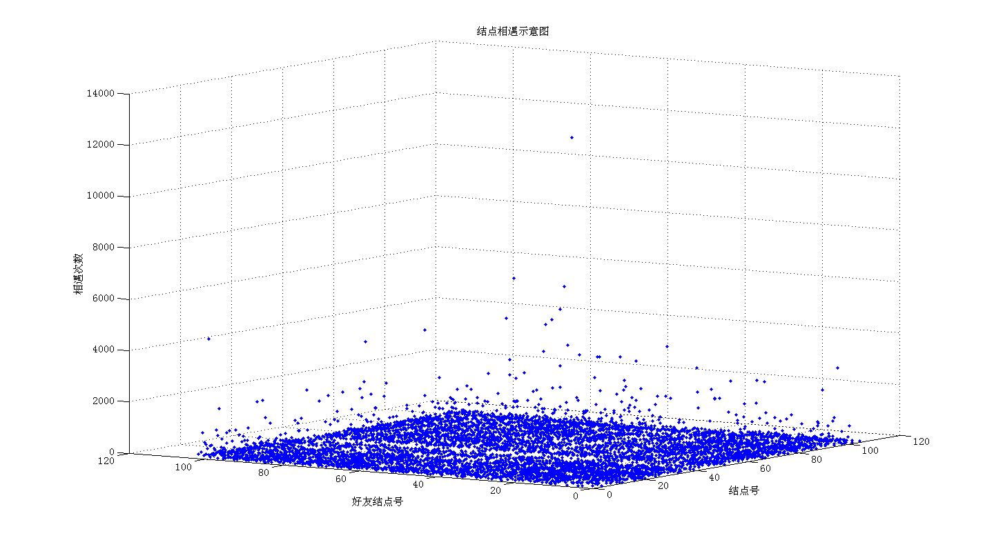
把好友关系蓝牙的扫描到的次数用用图形表示出来,程序写的比较乱便不贴上来了:
根据扫描到的次数进行好友排序的排序算法 ,这里是根据相遇时长进行排序,基于相遇频率的算法与之类似,对于连续扫描到相同mac 认为是一次相遇,略修改即可:
 1 function getdurationbluetoothfriends(S,Network)
 2
 3     disp('run scipt to get duration');
 4     [~,wS] = size(S);
 5     [~,wN] = size(Network.friends);
 6     limits = wN;  %94
 7     durationbluetooth = zeros(wS,wS);%这里储存的是 sub_index
 8     for n = 1:limits-1  %ws   1-93
 9         %sub_sort 是得到对应的 subject 号  1-106
10         device_mac = S(Network.sub_sort(n)).device_macs;
11         [~,t] = size(device_mac);   %cell
12         for m = 1:t
13             %添加一些什么方法     这里数据 是  1- m
14             EveryScan = device_mac{m}; %每一个cell 包含多个数据,所以还需要解析.
15              %每个output 还有多个数据,所以也要分离出来.
16             [hE,~] = size(EveryScan);
17             for r = 1:hE
18                 %在这里把每次扫描 的mac 与现有的mac 做比较 ,并加入到频率直方图中.
19                 %这里mac 获取应该没问题了.
20                 mac = EveryScan(r,1);
21                 sub_index = submacindex(mac,Network.sub_sort(n));
22                 if sub_index > 0
23                     %某个 subject 与某个  subject '相遇一次'  并计算次数
24                     durationbluetooth(Network.sub_sort(n),sub_index) = durationbluetooth(Network.sub_sort(n),sub_index)+1;
25                 end
26             end
27         end
28         disp(Network.sub_sort(n));
29     end
30     %对 frequencybluetooth  排序
31     %  行 为 project 号 列为对应好友 .
32     % 对 frequencybluetooth  数据进行排序
33     sortduration = zeros(wS,wS);%这里储存的是 sub_index
34     for i = 1:wS
35         [~,index] = sort(durationbluetooth(i,:),'descend');
36         sortduration(i,:) = index;
37     end
38
39     save 'sortduration' 'sortduration';
40     save 'durationbluetooth' 'durationbluetooth';
41
42     %用于获取根据传递 过来的 mac 的 subject 索引号
43     %  sub_index 为当前 mac 对应索引.
44     function index = submacindex(mac,currentIndex)
45         for index = 1:wS
46             if isempty(S(index).mac)   %1-93
47                 continue;
48             end
49             if index~=currentIndex && mac==S(index).mac
50                 return;
51             end
52         end
53         index = -1;   %表示数据不存在,非本实验已有的数据.
54     end
55 end
为了确保数据的有效,我简单写了个数据验证的 程序 :
 1 function checkdata(s)
 2     a = 61961024886;
 3     num = 0;
 4     data = s(3).device_macs;
 5     for n = 1:6100
 6         everyScan = data{n}; %每一个cell 包含多个数据,所以还需要解析.
 7         [h1,w1] = size(everyScan);
 8         for r = 1:h1
 9              mac = everyScan(r,1);
10              if mac == a
11                 index = char(num2str(n),'.',num2str(r),':');
12                 disp(index);
13                 num = num+1;
14                 disp(num2str(num));
15              end
16         end
17     end
18 end
看看这里统计的数据是否与上面排序时的频率是否相同,只需要取一个数据验证即可.
下面验证一下随机推荐的推荐效果.
根据上面好友排序算法生成的 sortduration 数据 和 原network数据 ,随机推荐算法:
%根据之前的生成的矩阵,与随机推荐做比较,并绘图
%这里先实现随机推荐,观察推荐好友数与 命中 个数的关系,正常情况下应该近似线性关系.
function recommendfriends(Sortfreq,Network)
     [~,wN] = size(Network.friends);
     [~,wS] = size(Sortfreq);
     relations = zeros(1,wS);


     %推荐好友的 个数从  1 - 106
     for m = 1:wS  %随机选择  m个好友,计算其命中个数
         randomHit = 0;

         r=randperm(wS);%生成1到106的随机排列
         selectedMatrix = r(1:m); %选择推荐  m 个好友 ,这里是随机推荐 是一维矩阵.
         %n 为对应subject  索引,非真正索引.
         for n = 1:wN-1      %1-93  对应   3-106
             % 3-106
             subjectIndex =  Network.sub_sort(n);  %subjectIndex为真实索引.
             randomHit =randomHit + hits(n,selectedMatrix);
         end
         % 储存 randomHit  与 对应 m 值 .
         relations(m) = randomHit;
     end
     save 'relations' 'relations';
     %绘图

     %数据做平滑处理.
     smoothData = smooth(relations,5);
     %plot(1:wS,smoothData(1:wS));
     plot(1:wS,smoothData(1:wS),'r*');
    %传入参数 ,
    function value = hits(n,selectedMatrix)
        value = 0;
        for i = 1:wN-1   %1- 93
            if Network.friends(n,i) >= 1
                realInex = Network.sub_sort(i);   %1- 106
                if any(selectedMatrix == realInex)   %矩阵中包含.realInex
                    value = value+1;
                end
            end
        end
    end %子函数
%最外部函数
end
因为数据的稀疏性,我简单做了smooth处理,感觉好很多.其结果如图:
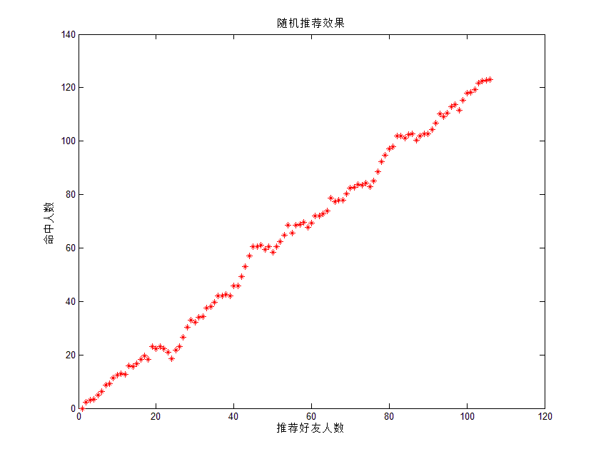
简单说明一下,为了验证推荐算法的有效性,我这里只做与随机推荐的对比.这里用命中数进行衡量,由于真实数据中,好友关系比较稀疏,统计的好友共有125个数据,
对于每个人,其推荐的好友越多其越是能够命中其原有的真实好友,所以在不采用任何算法的基础之上,其推荐好友人数与命中人数成线性关系 .
推荐比较图:
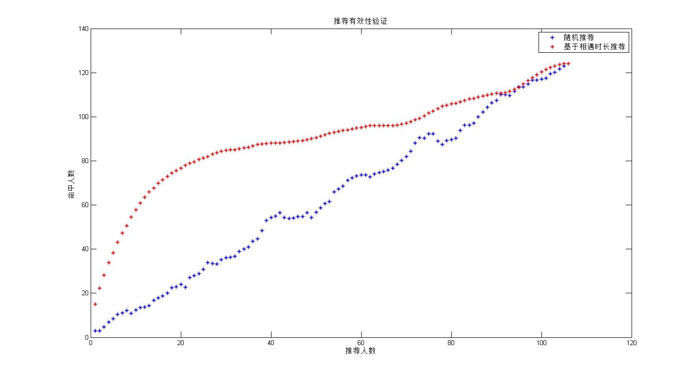
进行基于相遇时长和 相遇频率的实验,结果如图,看来基本没有什么差异,

实验总算完成了,和当初预想的一样,基于时长的推荐在开始处会一相对好的推荐结果,当推荐的人数增加,其逐渐等同于随机推荐.
为了做实验,生成了好多子数据,有需要的可以邮箱.本文程序供大家参考,请误抄袭.

 浙公网安备 33010602011771号