

从头开始使用梯度下降优化在Python中实现单变量多项式回归(后续3)
多项式回归
在涉及单个特征或变量的回归的预测分析问题(称为单变量回归)中,多项式回归是回归分析的重要变体,主要充当线性回归方面的性能提升。在本文中,我将介绍多项式回归,从零开始的Python实现以及在实际问题和性能分析上的应用。
如前缀“多项式”所示,机器学习算法的相应假设是多项式或多项式方程式。因此,这可以是任意程度的,例如如果假设是一阶多项式,则它是一个线性方程,因此称为线性回归;如果假设是二阶多项式,则它是一个二次方程,如果3次多项式,则它是一个三次方程式,依此类推。因此,可以说:
“ 线性回归是多项式回归的适当子集或特殊情况,因此多项式回归也称为广义回归 ”
多项式回归的假设如下:
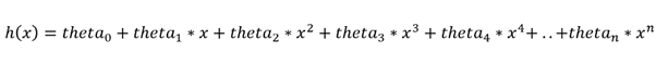
其中theta_0,theta_1,theta_2,theta_3,....,theta_n是参数,x是单个特征或变量
其中theta_0,theta_1,theta_2,theta_3,....,theta_n是参数,x是单个特征或变量
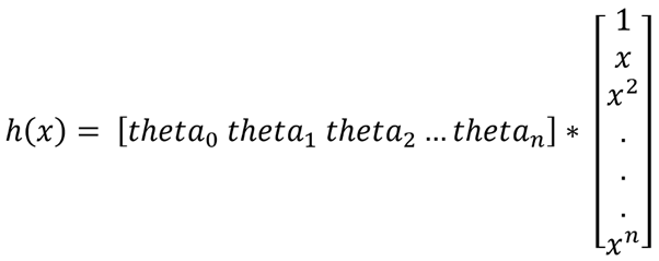
上述假设也可以用矩阵乘法格式或矢量代数表示为:
在这里,还有一个与假设相关的成本函数,取决于参数theta_0,theta_1,theta_2,theta_3,....,theta_n。
一般而言,广义回归的成本函数如下:
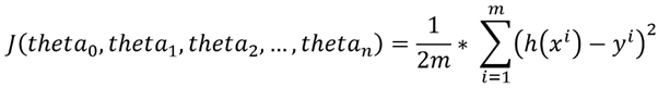
因此,这些参数theta_0,theta_1,theta_2,...,theta_n必须采用这样的值,对于这些值,成本函数(或简称为cost)达到其可能的最小值。换句话说,需要找出成本函数的最小值。
批梯度下降可以用作优化功能。
使用批次梯度下降实现多项式回归:
通过创建执行不同操作的3个模块来完成该实现。
=> hypothesis():在给定theta(theta_0,theta_1,theta_2,theta_3,....,theta_n),特征X和多项式回归(n中的多项式次数)的情况下,该函数计算并输出目标变量的假设值)作为输入。下面给出了hypothesis()的实现:
def hypothesis(theta, X, n):
h = np.ones((X.shape[0],1))
theta = theta.reshape(1,n+1)
for i in range(0,X.shape[0]):
x_array = np.ones(n+1)
for j in range(0,n+1):
x_array[j] = pow(X[i],j)
x_array = x_array.reshape(n+1,1)
h[i] = float(np.matmul(theta, x_array))
h = h.reshape(X.shape[0])
return h
=> BGD():此函数执行批量梯度下降算法,并采用theta的当前值(theta_0,theta_1,…,theta_n),学习率(alpha),迭代次数(num_iters),假设值列表所有样本(h),特征集(X),目标变量集(y)和多项式回归中的多项式度(n)作为输入,并输出优化的theta(theta_0,theta_1,theta_2,theta_3,…,theta_n),theta_history (包含每次迭代theta值的列表),最后是成本历史记录(cost),其中包含所有迭代中成本函数的值。BGD()的实现如下:
def BGD(theta, alpha, num_iters, h, X, y, n):
theta_history = np.ones((num_iters,n+1))
cost = np.ones(num_iters)
for i in range(0,num_iters):
theta[0] = theta[0] — (alpha/X.shape[0]) * sum(h — y)
for j in range(1,n+1):
theta[j]=theta[j]-(alpha/X.shape[0])*sum((h-y)*pow(X,j))
theta_history[i] = theta
h = hypothesis(theta, X, n)
cost[i] = (1/X.shape[0]) * 0.5 * sum(np.square(h — y))
theta = theta.reshape(1,n+1)
return theta, theta_history, cost
=> poly_regression():它是采用功能集(X),目标变量集(y),学习率(alpha),多项式回归中多项式的阶数(n)和迭代次数(num_iters)的主要函数。作为输入并输出最终优化的theta,即[ theta_0,theta_1,theta_2,theta_3,…。,theta_n ] 的值,在批量梯度下降之后,成本函数几乎达到了最小值,theta_history存储每次迭代的theta值而成本则存储每次迭代的成本价值。
def poly_regression(X, y, alpha, n, num_iters):
# initializing the parameter vector…
theta = np.zeros(n+1)
# hypothesis calculation….
h = hypothesis(theta, X, n)
# returning the optimized parameters by Gradient Descent
theta,theta_history,cost=BGD(theta,alpha,num_iters,h, X, y, n)
return theta, theta_history, cost
问题陈述:“ 根据城市人口,使用多项式回归分析和预测公司的利润”
data = np.loadtxt(‘data1.txt’, delimiter=’,’)
X_train = data[:,0] #the feature_set
y_train = data[:,1] #the labels
# calling the principal function with learning_rate = 0.0001 and
# n = 2(quadratic_regression) and num_iters = 300000
theta,theta_history,cost=poly_regression(X_train,y_train,0.00001,2,300000)

多项式回归后的theta
散点图中theta的可视化:
可以在散点图中完成获得的theta的回归线可视化:
import matplotlib.pyplot as plt
training_predictions = hypothesis(theta, X_train, 2)
scatter = plt.scatter(X_train, y_train, label=”training data”) regression_line = plt.plot(X_train, training_predictions
,label=”polynomial (degree 2) regression”)
plt.legend()
plt.xlabel(‘Population of City in 10,000s’)
plt.ylabel(‘Profit in $10,000s’)
回归线可视化结果为:

二次回归后的回归线可视化
而且,在逐次迭代的批次梯度下降过程中,成本已降低。借助“线曲线”可以显示成本的降低。
import matplotlib.pyplot as plt
cost = list(cost)
n_iterations = [x for x in range(1,300001)]
plt.plot(n_iterations, cost)
plt.xlabel(‘No. of iterations’)
plt.ylabel(‘Cost’)
线曲线显示为:

二次回归中使用BGD的成本最小化的线曲线表示
现在,必须进行模型性能分析以及多项式回归与线性回归(具有相同迭代次数)的比较。
data = np.loadtxt(‘data1.txt’, delimiter=’,’)
X_train = data[:,0] #the feature_set
y_train = data[:,1] #the labels
# calling the principal function with learning_rate = 0.0001 and
# num_iters = 300000
theta,theta_0,theta_1,cost=linear_regression(X_train,y_train,
0.0001,300000)

线性回归后的θ
散点图中theta的可视化:
可以在散点图中完成获得的theta的回归线可视化:
import matplotlib.pyplot as plt
training_predictions = hypothesis(theta, X_train)
scatter = plt.scatter(X_train, y_train, label=”training data”)
regression_line = plt.plot(X_train, training_predictions
, label=”linear regression”)
plt.legend()
plt.xlabel(‘Population of City in 10,000s’)
plt.ylabel(‘Profit in $10,000s’)
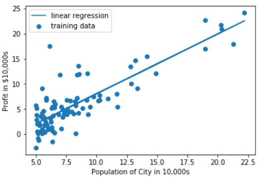
线性回归后的回归线可视化
而且,在逐次迭代的批次梯度下降过程中,成本已降低。借助“线曲线”可以显示成本的降低。
import matplotlib.pyplot as plt
cost = list(cost)
n_iterations = [x for x in range(1,300001)]
plt.plot(n_iterations, cost)
plt.xlabel(‘No. of iterations’)
plt.ylabel(‘Cost’)
线曲线显示为:

线性回归中使用BGD的成本最小化的线曲线表示
性能分析(使用BGD优化的线性回归与二次回归):

但是在这里,使用批梯度下降优化技术,我们得到的线性回归在所有方面都优于多项式(二次)回归。但是,实际上,总是多项式(高阶或广义)回归的性能优于线性回归。尽管使用了BGD,但由于BGD优化本身存在一些缺陷,我们无法获得与命题匹配的实验结果。还有另一种优化或找到多项式(也是线性)回归中的成本函数最小值的方法,称为OLS(普通最小二乘)或正态方程法。
使用OLS,可以清楚地证明多项式(在此实验中为Quadratic)的性能优于线性回归。除单变量问题外,多项式回归还可以使用适当的特征工程技术在多变量问题(多个特征)中使用。
这就是多项式回归。

 浙公网安备 33010602011771号