

从头开始使用梯度下降优化在Python中实现单变量多项式回归
回归是对特征空间中的数据或数据点进行连续分类的一种方法。弗朗西斯·高尔顿(Francis Galton)于1886年发明了回归线的用法[1]。
线性回归
这是多项式回归的一种特殊情况,其中假设中多项式的阶数为1。本文的后半部分讨论了一般多项式回归。顾名思义,“线性”是指有关机器学习算法的假设本质上是线性的,或者只是线性方程式。是的!这确实是一个线性方程。在单变量线性回归中,存在目标变量所依赖的单个要素或变量。
单变量线性回归的假设如下:
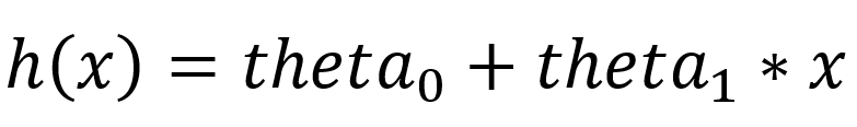
上述假设也可以用矩阵乘法格式或矢量代数表示为:
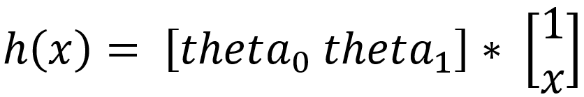
与假设相关的成本函数取决于参数theta_0和theta_1。
通常,线性回归的成本函数如下:

现在,这两个参数theta_0和theta_1必须采用这样的值,以使该成本函数的值(即成本)采用可能的最小值。因此,现在的基本目标是找到成本最小的theta_0和theta_1值,或者简单地找到成本函数的最小值。
梯度下降法是最著名的凸优化技术之一,利用该技术可以找到最小的函数。梯度下降算法如下:

梯度下降有两种方法:
- 随机梯度下降
- 批次梯度下降
使用随机梯度下降实现线性回归:
在随机梯度下降中,运行梯度下降算法,一次从数据集中获取一个实例。
通过创建3个具有不同操作的模块来完成实现:
=> hypothesis():该函数在给定theta(theta_0和theta_1)和Feature X作为输入的情况下,计算并输出目标变量的假设值。下面给出了hypothesis()的实现:
def hypothesis(theta, X):
h = np.ones((X.shape[0],1))
for i in range(0,X.shape[0]):
x = np.concatenate((np.ones(1), np.array([X[i]])), axis = 0)
h[i] = float(np.matmul(theta, x))
h = h.reshape(X.shape[0])
return h
=> SGD():该函数执行随机梯度下降算法,采用theta_0和theta_1的当前值,alpha,迭代次数(num_iters),假设值(h),特征集(X)和目标变量集( y)作为输入,并在以实例为特征的每次迭代中输出优化的theta(theta_0和theta_1)。SGD()的实现如下:
def SGD(theta, alpha, num_iters, h, X, y):
for i in range(0,num_iters):
theta[0] = theta[0] - (alpha) * (h - y)
theta[1] = theta[1] - (alpha) * ((h - y) * X)
h = theta[1]*X + theta[0]
return theta
=> sgd_linear_regression():该主要函数将特征集(X),目标变量集(y),学习率和迭代次数(num_iters)作为输入,并输出最终的优化theta,即theta_0的值和theta_1,其成本函数在随机梯度下降之后几乎达到最小值。
def sgd_linear_regression(X, y, alpha, num_iters):
# initializing the parameter vector...
theta = np.zeros(2)
# hypothesis calculation....
h = hypothesis(theta, X)
# returning the optimized parameters by Gradient Descent...
for i in range(0, X.shape[0]):
theta = SGD(theta,alpha,num_iters,h[i],X[i],y[i])
theta = theta.reshape(1, 2)
return theta
问题陈述:“ 根据城市人口,使用线性回归分析和预测公司的利润 ”
数据读入Numpy数组:
data = np.loadtxt('data1.txt', delimiter=',')
X_train = data[:,0] #the feature_set
y_train = data[:,1] #the labels
数据可视化:可以使用散点图可视化数据集:
import matplotlib.pyplot as plt
plt.scatter(X_train, y_train)
plt.xlabel('Population of City in 10,000s')
plt.ylabel('Profit in $10,000s')
散点图数据可视化看起来像-
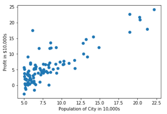
散点图
使用3-模块线性回归-SGD:
#调用与主要功能learning_rate = 0.0001和
#num_iters = 100000
 THETA = sgd_linear_regression(X_train,y_train,0.0001,100000)
theta输出结果为:

SGD之后的theta
散点图中theta的可视化:
可以在散点图中完成获得的theta的回归线可视化:
import matplotlib.pyplot as plt
# getting the predictions...
training_predictions = hypothesis(theta, X_train)
scatter = plt.scatter(X_train, y_train, label="training data")
regression_line = plt.plot(X_train, training_predictions
, label="linear regression")
plt.legend()
plt.xlabel('Population of City in 10,000s')
plt.ylabel('Profit in $10,000s')
回归线可视化结果为:

SGD之后的回归线可视化

 浙公网安备 33010602011771号