改善深层神经网络-week1编程题(GradientChecking)
1. Gradient Checking
你被要求搭建一个Deep Learning model来检测欺诈,每当有人付款,你想知道是否该支付可能是欺诈,例如该用户的账户可能已经被黑客掉。
但是,反向传播实现起来非常有挑战,并且有时有一些bug,因为这是一个mission-critical应用,你公司老板想让十分确定,你实现的反向传播是正确的。你需要用“gradient checking”来证明你的反向传播是正确的。
# Packages
import numpy as np
from testCases import *
from gc_utils import sigmoid, relu, dictionary_to_vector, vector_to_dictionary, gradients_to_vector
1.1 gradient checking 如何工作?
Backpropagation 计算梯度(the gradients) \(\frac{\partial J}{\partial \theta}\), \(\theta\)代表着模型的参数,\(J\) 是使用前向传播和你的loss function来计算的。
前向传播十分容易,因此你使用计算 \(J\) 的代码 来确认计算 \(\frac{\partial J}{\partial \theta}\) 的代码
我们来看一下derivative (or gradient)的定义:
接下来:
- \(\frac{\partial J}{\partial \theta}\) 是你想要确保计算正确的
- 你可以计算\(J(\theta + \varepsilon)\) and \(J(\theta - \varepsilon)\)(这个例子中\(\theta\)是一个实数)。(已知J是正确的)
我们要使用公式(1) 和一个很小的数 \(\varepsilon\) 来保证你计算 \(\frac{\partial J}{\partial \theta}\) 的代码是正确的。
2. 1-dimensional gradient checking
只考虑一元线性函数 \(J(\theta) = \theta x\). The model contains only a single real-valued parameter \(\theta\), and takes \(x\) as input.
You will implement code to compute \(J(.)\) and its derivative \(\frac{\partial J}{\partial \theta}\). You will then use gradient checking to make sure your derivative computation for \(J\) is correct.
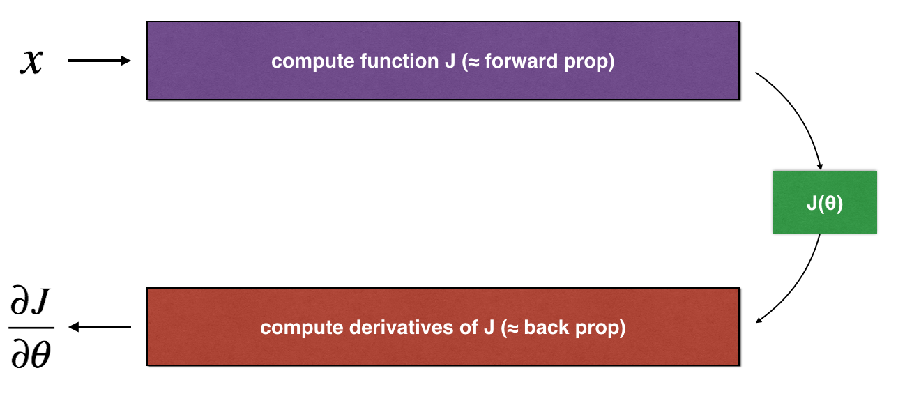
上图展示了关键的计算步骤: 首先开始于 \(x\), 随后评估 \(J(x)\) ("forward propagation"). 然后计算 the derivative \(\frac{\partial J}{\partial \theta}\) ("backward propagation").
Exercise: 实现这个简单函数的 "forward propagation" and "backward propagation" . I.e., 计算 \(J(.)\) ("forward propagation") 和 它关于 \(\theta\) 的导数("backward propagation"), 在两个函数里。
# GRADED FUNCTION: forward_propagation

def forward_propagation(x, theta):
    """
    Implement the linear forward propagation (compute J) presented in Figure 1 (J(theta) = theta * x)

    Arguments:
    x -- a real-valued input
    theta -- our parameter, a real number as well

    Returns:
    J -- the value of function J, computed using the formula J(theta) = theta * x
    """

    ### START CODE HERE ### (approx. 1 line)
    J = theta * x
    ### END CODE HERE ###

    return J
测试:
x, theta = 2, 4
J = forward_propagation(x, theta)
print ("J = " + str(J))
J = 8
Exercise: 现在,实现图1中反向传播(导数计算)步骤:计算 \(J(\theta) = \theta x\) 关于 \(\theta\) 的导数. 用 \(dtheta = \frac { \partial J }{ \partial \theta} = x\) 来保存你做的计算。
# GRADED FUNCTION: backward_propagation

def backward_propagation(x, theta):
    """
    Computes the derivative of J with respect to theta (see Figure 1).

    Arguments:
    x -- a real-valued input
    theta -- our parameter, a real number as well

    Returns:
    dtheta -- the gradient of the cost with respect to theta
    """

    ### START CODE HERE ### (approx. 1 line)
    dtheta = x
    ### END CODE HERE ###

    return dtheta
测试
x, theta = 2, 4
dtheta = backward_propagation(x, theta)
print ("dtheta = " + str(dtheta))
dtheta = 2
Exercise: 为了显示 backward_propagation() 函数是正确计算 the gradient \(\frac{\partial J}{\partial \theta}\), 让我们实现 gradient checking.
Instructions:
- 首先,计算 "gradapprox" 使用公式(1)和 一个很小的值 \(\varepsilon\).遵循以下步骤:
- \(\theta^{+} = \theta + \varepsilon\)
- \(\theta^{-} = \theta - \varepsilon\)
- \(J^{+} = J(\theta^{+})\)
- \(J^{-} = J(\theta^{-})\)
- \(gradapprox = \frac{J^{+} - J^{-}}{2 \varepsilon}\)
- 然后,使用backward propagation计算gradient , 并存储结果到变量 "grad"
- 最后, 计算 "gradapprox" 和 the "grad" 的相对偏差,使用下列公式:
你需要三个步骤来计算这个公式:
- 1'. compute the numerator(分子) using np.linalg.norm(...)
- 2'. compute the denominator(分母). You will need to call np.linalg.norm(...) twice.
- 3'. divide them.
- 如果这个 difference 非常小 (小于 \(10^{-7}\)), gradient计算正确. 否则,错误.
# GRADED FUNCTION: gradient_check

def gradient_check(x, theta, epsilon = 1e-7):
    """
    Implement the backward propagation presented in Figure 1.

    Arguments:
    x -- a real-valued input
    theta -- our parameter, a real number as well
    epsilon -- tiny shift to the input to compute approximated gradient with formula(1)

    Returns:
    difference -- difference (2) between the approximated gradient and the backward propagation gradient
    """

    # Compute gradapprox using left side of formula (1). epsilon is small enough, you don't need to worry about the limit.
    ### START CODE HERE ### (approx. 5 lines)
    thetaplus = theta + epsilon
    thetaminus = theta - epsilon
    J_plus = forward_propagation(x, thetaplus)
    J_minus = forward_propagation(x, thetaminus)
    gradapprox = (J_plus - J_minus) / (2. * epsilon)
    ### END CODE HERE ###

    # Check if gradapprox is close enough to the output of backward_propagation()
    ### START CODE HERE ### (approx. 1 line)
    grad = backward_propagation(x, theta)
    ### END CODE HERE ###

    ### START CODE HERE ### (approx. 1 line)
    numerator = np.linalg.norm(grad - gradapprox)
    denominator = np.linalg.norm(grad) + np.linalg.norm(gradapprox)
    difference = numerator / denominator
    ### END CODE HERE ###

    if difference < 1e-7:
        print ("The gradient is correct!")
    else:
        print ("The gradient is wrong!")

    return difference
x, theta = 2, 4
difference = gradient_check(x, theta)
print("difference = " + str(difference))
The gradient is correct!
difference = 2.919335883291695e-10
上述计算检验正确。即,可以正确的计算反向传播。
现在,你的 cost function \(J\) has more than a single 1D input。当你训练一个神经网络,\(\theta\) 事实上由multiple matrices \(W^{[l]}\) and biases \(b^{[l]}\)组成,知道如何 梯度检验 高维度输入 非常重要。
3. N-dimensional gradient checking
下图描述了你的欺诈检测的前向和反向传播的模型:
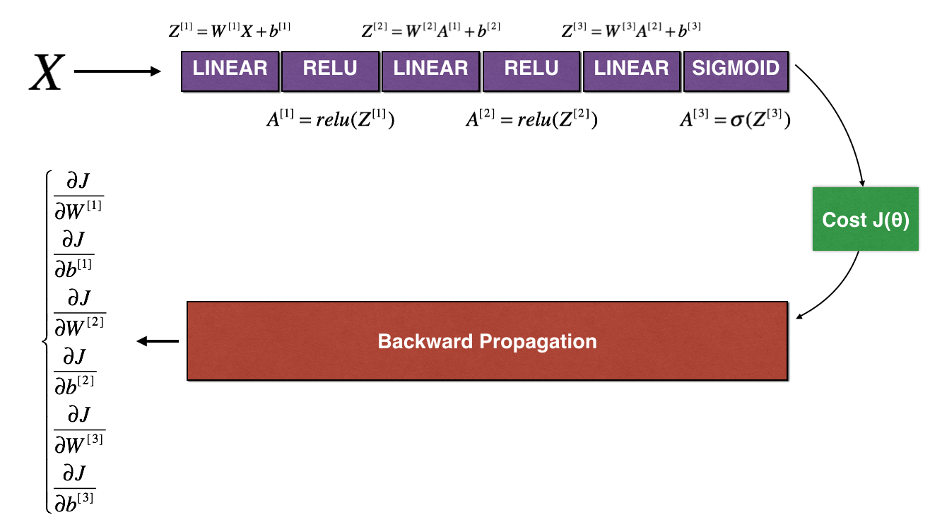
*LINEAR -> RELU -> LINEAR -> RELU -> LINEAR -> SIGMOID*
下面实现forward propagation and backward propagation.
def forward_propagation_n(X, Y, parameters):
    """
    Implements the forward propagation (and computes the cost) presented in Figure 3.

    Arguments:
    X -- training set for m examples
    Y -- labels for m examples
    parameters -- python dictionary containing your parameters "W1", "b1", "W2", "b2", "W3", "b3":
                    W1 -- weight matrix of shape (5, 4)
                    b1 -- bias vector of shape (5, 1)
                    W2 -- weight matrix of shape (3, 5)
                    b2 -- bias vector of shape (3, 1)
                    W3 -- weight matrix of shape (1, 3)
                    b3 -- bias vector of shape (1, 1)

    Returns:
    cost -- the cost function (logistic cost for one example)
    """

    # retrieve parameters
    m = X.shape[1]
    W1 = parameters["W1"]
    b1 = parameters["b1"]
    W2 = parameters["W2"]
    b2 = parameters["b2"]
    W3 = parameters["W3"]
    b3 = parameters["b3"]

    # LINEAR -> RELU -> LINEAR -> RELU -> LINEAR -> SIGMOID
    Z1 = np.dot(W1, X) + b1
    A1 = relu(Z1)
    Z2 = np.dot(W2, A1) + b2
    A2 = relu(Z2)
    Z3 = np.dot(W3, A2) + b3
    A3 = sigmoid(Z3)

    # Cost
    logprobs = np.multiply(-np.log(A3),Y) + np.multiply(-np.log(1 - A3), 1 - Y)
    cost = 1./m * np.sum(logprobs)

    cache = (Z1, A1, W1, b1, Z2, A2, W2, b2, Z3, A3, W3, b3)

    return cost, cache
Now, run backward propagation.
def backward_propagation_n(X, Y, cache):
    """
    Implement the backward propagation presented in figure 2.

    Arguments:
    X -- input datapoint, of shape (input size, 1)
    Y -- true "label"
    cache -- cache output from forward_propagation_n()

    Returns:
    gradients -- A dictionary with the gradients of the cost with respect to each parameter, activation and pre-activation variables.
    """

    m = X.shape[1]
    (Z1, A1, W1, b1, Z2, A2, W2, b2, Z3, A3, W3, b3) = cache

    dZ3 = A3 - Y
    dW3 = 1./m * np.dot(dZ3, A2.T)
    db3 = 1./m * np.sum(dZ3, axis=1, keepdims=True)


    dA2 = np.dot(W3.T, dZ3)
    dZ2 = np.multiply(dA2, np.int64(A2 > 0))
    dW2 = 1./m * np.dot(dZ2, A1.T) * 2                  # 这里故意写错
    db2 = 1./m * np.sum(dZ2, axis=1, keepdims = True)

    dA1 = np.dot(W2.T, dZ2)
    dZ1 = np.multiply(dA1, np.int64(A1 > 0))
    dW1 = 1./m * np.dot(dZ1, X.T)
    db1 = 4./m * np.sum(dZ1, axis=1, keepdims = True)   # 这里故意写错

    gradients = {"dZ3": dZ3, "dW3": dW3, "db3": db3,
                 "dA2": dA2, "dZ2": dZ2, "dW2": dW2, "db2": db2,
                 "dA1": dA1, "dZ1": dZ1, "dW1": dW1, "db1": db1}

    return gradients
下面进行梯度检验来确保你的梯度是正确的.
gradient checking 如何工作?.
As in 1) and 2), you want to compare "gradapprox" to the gradient computed by backpropagation. The formula is still:
但是, \(\theta\) 不再是标量. 而是一个叫 "parameters"的字典. 下面实现一个 "dictionary_to_vector()"(字典转向量). 它将"parameters" dictionary 转换成名为"values"的vector, 通过 reshaping all parameters (W1, b1, W2, b2, W3, b3) into vectors and concatenating(连接) them 获得.
The inverse function is "vector_to_dictionary"(向量转字典) which outputs back the "parameters" dictionary.
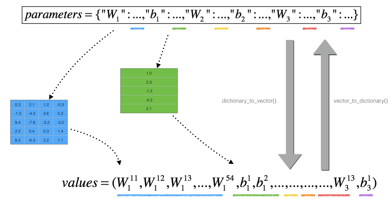
You will need these functions in gradient_check_n()
We have also converted the "gradients" dictionary into a vector "grad" using gradients_to_vector(). You don't need to worry about that.
Exercise: Implement gradient_check_n().
Instructions: 这里的伪代码(pseudo-code)将帮助你实现梯度检测(the gradient check).
For each i in num_parameters:
- To compute
J_plus[i]:- Set \(\theta^{+}\) to
np.copy(parameters_values)(深拷贝) - Set \(\theta^{+}_i\) to \(\theta^{+}_i + \varepsilon\)
- Calculate \(J^{+}_i\) using to
forward_propagation_n(x, y, vector_to_dictionary(\(\theta^{+}\))).
- Set \(\theta^{+}\) to
- To compute
J_minus[i]: do the same thing with \(\theta^{-}\) - Compute \(gradapprox[i] = \frac{J^{+}_i - J^{-}_i}{2 \varepsilon}\)
Thus, you get a vector gradapprox, where gradapprox[i] is an approximation of the gradient with respect to parameter_values[i]. You can now compare this gradapprox vector to the gradients vector from backpropagation. Just like for the 1D case (Steps 1', 2', 3'), compute:
# GRADED FUNCTION: gradient_check_n

def gradient_check_n(parameters, gradients, X, Y, epsilon = 1e-7):
    """
    Checks if backward_propagation_n computes correctly the gradient of the cost output by forward_propagation_n

    Arguments:
    parameters -- python dictionary containing your parameters "W1", "b1", "W2", "b2", "W3", "b3":
    grad -- output of backward_propagation_n, contains gradients of the cost with respect to the parameters.
    x -- input datapoint, of shape (input size, 1)
    y -- true "label"
    epsilon -- tiny shift to the input to compute approximated gradient with formula(1)

    Returns:
    difference -- difference (2) between the approximated gradient and the backward propagation gradient
    """

    # Set-up variables
#     print(parameters)
    parameters_values, _ = dictionary_to_vector(parameters)    # 将字典转换成向量
#     print(parameters_values, i)                              # (W1, b1, W2, b2, .....) (注:此处W1,b1都转换成了向量)
    grad = gradients_to_vector(gradients)           # 梯度转换成向量
    num_parameters = parameters_values.shape[0]     # 所有参数个数
    J_plus = np.zeros((num_parameters, 1))          # 初始化为 (num, 1)的向量
    J_minus = np.zeros((num_parameters, 1))
    gradapprox = np.zeros((num_parameters, 1))

    # Compute gradapprox
    for i in range(num_parameters):                 # 遍历所有参数,每个参数都求一遍 gradapprox,很费时间

        # Compute J_plus[i]. Inputs: "parameters_values, epsilon". Output = "J_plus[i]".
        # "_" is used because the function you have to outputs two parameters but we only care about the first one
        ### START CODE HERE ### (approx. 3 lines)
        thetaplus = np.copy(parameters_values)
        thetaplus[i, 0] += epsilon
        # Step 2
        J_plus[i], _ = forward_propagation_n(X, Y, vector_to_dictionary(thetaplus))      # Step 3
        ### END CODE HERE ###

        # Compute J_minus[i]. Inputs: "parameters_values, epsilon". Output = "J_minus[i]".
        ### START CODE HERE ### (approx. 3 lines)
        thetaminus = np.copy(parameters_values)                   # Step 1
        thetaminus[i, 0] -= epsilon                               # Step 2
        J_minus[i], _ = forward_propagation_n(X, Y, vector_to_dictionary(thetaminus))   # Step 3
        ### END CODE HERE ###

        # Compute gradapprox[i]
        ### START CODE HERE ### (approx. 1 line)
        gradapprox[i] = (J_plus[i] - J_minus[i]) / (2. * epsilon)
        ### END CODE HERE ###

    # Compare gradapprox to backward propagation gradients by computing difference.
    ### START CODE HERE ### (approx. 1 line)
    numerator = np.linalg.norm(grad - gradapprox)                               # Step 1'
    denominator = np.linalg.norm(grad) + np.linalg.norm(gradapprox)             # Step 2'
    difference = numerator / denominator

    if difference > 1.2e-7:
        print ("\033[93m" + "There is a mistake in the backward propagation! difference = " + str(difference) + "\033[0m")
    else:
        print ("\033[92m" + "Your backward propagation works perfectly fine! difference = " + str(difference) + "\033[0m")

    return difference
X, Y, parameters = gradient_check_n_test_case()

cost, cache = forward_propagation_n(X, Y, parameters)
gradients = backward_propagation_n(X, Y, cache)
difference = gradient_check_n(parameters, gradients, X, Y)
可以看出,在 backward_propagation_n代码中有一些错误。
现在,我们修复这个错误,再来运行一下上面代码:
    dA2 = np.dot(W3.T, dZ3)
    dZ2 = np.multiply(dA2, np.int64(A2 > 0))
#     dW2 = 1./m * np.dot(dZ2, A1.T) * 2                  # 这里故意写错
    dW2 = 1./m * np.dot(dZ2, A1.T)                       # 修复
    db2 = 1./m * np.sum(dZ2, axis=1, keepdims = True)

    dA1 = np.dot(W2.T, dZ2)
    dZ1 = np.multiply(dA1, np.int64(A1 > 0))
    dW1 = 1./m * np.dot(dZ1, X.T)
#     db1 = 4./m * np.sum(dZ1, axis=1, keepdims = True)   # 这里故意写错
    db1 = 1./m * np.sum(dZ1, axis=1, keepdims = True)   # 修复
重新运行 backward_propagation_n()
输出:
Your backward propagation works perfectly fine! difference = 1.1885552035482147e-07
Note
- Gradient Checking is slow! Approximating the gradient with \(\frac{\partial J}{\partial \theta} \approx \frac{J(\theta + \varepsilon) - J(\theta - \varepsilon)}{2 \varepsilon}\) 计算非常耗时. 因此, 我们在训练集上不是每一次迭代都运行梯度检测. 仅几次验证梯度是否正确,然后关掉它。
- Gradient Checking, 不能和dropout一起工作. 你可以关掉 dropout 再运行 the gradient check algorithm 来确保你的 backprop 是正确的, 然后再打开dropout.

 浙公网安备 33010602011771号