用神经网络拟合数据

1 神经元

从本质上讲，神经元不过是输入的线性变换（例如，输入乘以一个数[weight，权重]，再加上一个常数[偏置，bias]），然后再经过一个固定的非线性函数（称为激活函数）。

神经元：线性变换后再经过一个非线性函数

数学上，你可以将其写为 $o = f(wx + b)$

$o = f(wx + b)$

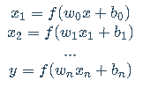
其中神经元层的输出将用作下一层的输入。请记住，这里的 $w0w_0w0 是一个矩阵，而 xxx 是一个向量！在此使用向量可使 w0w_0w0 容纳整个神经元层，而不仅仅是单个权重。$

激活函数：（深度）神经网络中最简单的单元是线性运算（缩放+偏移）然后紧跟一个激活函数。在你的上一个模型中有一个线性运算，而这个线性运算就是整个模型。激活函数的作用是将先前线性运算的输出聚集到给定范围内。

几个常见及不常见的激活函数：

2、PyTorch的nn模块

实例化nn.Linear并将其像一个函数一样进行调用

import torch.nn as nn

linear_model = nn.Linear(1, 1) # 参数: input size, output size, bias(默认True)
linear_model.weight   # 权重
linear_model.bias   # 偏差
linear_model.parameters() # 参数

nn中的任何模块都被编写成同时产生一个批次（即多个输入）的输出。因此，假设你需要对10个样本运行nn.Linear，则可以创建大小为 B x Nin 的输入张量，其中 B 是批次的大小，而 Nin 是输入特征的数量，然后在模型中同时运行：

x = torch.ones(10, 1)
linear_model(x)

现在更新原来的训练代码。首先，将之前的手工模型替换为nn.Linear(1,1)，然后将线性模型参数传递给优化器：

linear_model = nn.Linear(1, 1)
optimizer = optim.SGD(
    linear_model.parameters(),  # 之前，你需要自己创建参数并将其作为第一个参数传递给optim.SGD
    lr=1e-2)

用神经网络代替线性模型作为近似函数：

接下来我们将重新定义模型，并将所有其他内容（包括损失函数）保持不变。还是构建最简单的神经网络：一个线性模块然后是一个激活函数，最后将输入喂入另一个线性模块

# nn提供了一种通过nn.Sequential容器串联模块的简单方法：
seq_model = nn.Sequential(
            nn.Linear(1, 13),
            nn.Tanh(),
            nn.Linear(13, 1))
seq_model

from collections import OrderedDict

seq_model = nn.Sequential(OrderedDict([
    ('hidden_linear', nn.Linear(1, 8)),
    ('hidden_activation', nn.Tanh()),
    ('output_linear', nn.Linear(8, 1))
]))

seq_model

$o = f(wx + b)$

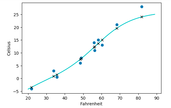
#!/usr/bin/env python
# coding: utf-8

# In[1]:


import torch
import torch.nn as nn
import torch.optim as optim

torch.set_printoptions(edgeitems=2)
torch.manual_seed(2020)


# In[2]:


t_c = [0.5,  14.0, 15.0, 28.0, 11.0,  8.0,  3.0, -4.0,  6.0, 13.0, 21.0]
t_u = [35.7, 55.9, 58.2, 81.9, 56.3, 48.9, 33.9, 21.8, 48.4, 60.4, 68.4]
t_c = torch.tensor(t_c).unsqueeze(1) # <1>
t_u = torch.tensor(t_u).unsqueeze(1) # <1>

t_u.shape


# In[3]:


n_samples = t_u.shape[0]
n_val = int(0.2 * n_samples)

shuffled_indices = torch.randperm(n_samples)

train_indices = shuffled_indices[:-n_val]
val_indices = shuffled_indices[-n_val:]

train_indices, val_indices


# In[8]:


t_u_train = t_u[train_indices]  # t_u里的测试集
t_c_train = t_c[train_indices]  # t_c对应t_u测试集的部分

t_u_val = t_u[val_indices]   # t_u里验证集
t_c_val = t_c[val_indices]   # t_c里对应t_u验证集的部分

t_un_train = 0.1 * t_u_train  # 相当于把t_u里的数据*0.1
t_un_val = 0.1 * t_u_val


# In[6]:


linear_model = nn.Linear(1, 1) # 参数: input size, output size, bias(默认True)
linear_model(t_un_val)


# In[9]:


# 现在你有一个具有一个输入和一个输出特征的nn.Linear实例，它需要一个权重
linear_model.weight


# In[10]:


# 一个偏差
linear_model.bias


# In[12]:


# 你可以用一些输入来调用这个模块
x = torch.ones(1)
linear_model(x)


# In[13]:


# nn中的任何模块都被编写成同时产生一个批次（即多个输入）的输出
x = torch.ones(10,1)
linear_model(x)


# In[14]:


# 这就是你要切换到使用nn.Linear所要做的。你需要将尺寸为 B 的输入reshape为 B x Nin，其中Nin为1。你可以使用unsqueeze轻松地做到这一点：
t_c = [0.5,  14.0, 15.0, 28.0, 11.0,  8.0,  3.0, -4.0,  6.0, 13.0, 21.0]
t_u = [35.7, 55.9, 58.2, 81.9, 56.3, 48.9, 33.9, 21.8, 48.4, 60.4, 68.4]
t_c = torch.tensor(t_c).unsqueeze(1) # <1>
t_u = torch.tensor(t_u).unsqueeze(1) # <1>

t_u.shape


# In[15]:


linear_model = nn.Linear(1, 1)
optimizer = optim.SGD(
    linear_model.parameters(),
    lr=1e-2)


# In[16]:


print(linear_model.parameters())
print(list(linear_model.parameters()))


# In[17]:


def training_loop(n_epochs, optimizer, model, loss_fn, 
                  t_u_train, t_u_val, t_c_train, t_c_val):
    for epoch in range(1, n_epochs + 1):
        t_p_train = model(t_un_train)
        loss_train = loss_fn(t_p_train, t_c_train)

        t_p_val = model(t_un_val)
        loss_val = loss_fn(t_p_val, t_c_val)

        optimizer.zero_grad()
        loss_train.backward()
        optimizer.step()

        if epoch == 1 or epoch % 1000 == 0:
            print('Epoch %d, Training loss %.4f, Validation loss %.4f' % (
                    epoch, float(loss_train), float(loss_val)))


# In[18]:


linear_model = nn.Linear(1, 1)
optimizer = optim.SGD(linear_model.parameters(), lr=1e-2)

training_loop(
    n_epochs = 3000,
    optimizer = optimizer,
    model = linear_model,
    loss_fn = nn.MSELoss(), # 不再使用自己定义的loss
    t_u_train = t_un_train,
    t_u_val = t_un_val,
    t_c_train = t_c_train,
    t_c_val = t_c_val)

print()
print(linear_model.weight)
print(linear_model.bias)

# nn提供了一种通过nn.Sequential容器串联模块的简单方法：
# In[19]:


seq_model = nn.Sequential(
            nn.Linear(1, 13),
            nn.Tanh(),
            nn.Linear(13, 1))
seq_model


# In[20]:


[param.shape for param in seq_model.parameters()]


# In[21]:


for name, param in seq_model.named_parameters():
    print(name, param.shape)

# Sequential还可以接受OrderedDict作为参数，这样就可以给Sequential的每个模块命名：
# In[22]:


from collections import OrderedDict

seq_model = nn.Sequential(OrderedDict([
    ('hidden_linear', nn.Linear(1, 8)),
    ('hidden_activation', nn.Tanh()),
    ('output_linear', nn.Linear(8, 1))
]))

seq_model


# In[23]:


for name, param in seq_model.named_parameters():
    print(name, param.shape)


# In[24]:


optimizer = optim.SGD(seq_model.parameters(), lr=1e-3) # 为了稳定性调小了梯度

training_loop(
    n_epochs = 5000,
    optimizer = optimizer,
    model = seq_model,
    loss_fn = nn.MSELoss(),
    t_u_train = t_un_train,
    t_u_val = t_un_val,
    t_c_train = t_c_train,
    t_c_val = t_c_val)

print('output', seq_model(t_un_val))
print('answer', t_c_val)
print('hidden', seq_model.hidden_linear.weight.grad)


# In[26]:


from matplotlib import pyplot as plt

t_range = torch.arange(20., 90.).unsqueeze(1)

fig = plt.figure(dpi=100)
plt.xlabel("Fahrenheit")
plt.ylabel("Celsius")
plt.plot(t_u.numpy(), t_c.numpy(), 'o')
plt.plot(t_range.numpy(), seq_model(0.1 * t_range).detach().numpy(), 'c-')
plt.plot(t_u.numpy(), seq_model(0.1 * t_u).detach().numpy(), 'kx')
plt.show()


# In[ ]:

posted @ 2021-03-10 09:25 +D 阅读(887) 评论(0) 编辑收藏举报

会员力量，点亮园子希望

刷新页面返回顶部

D

剑尚未配妥，出门已是江湖

用神经网络拟合数据

1 神经元

2、PyTorch的nn模块

$o = f(wx + b)$

公告

D

剑尚未配妥，出门已是江湖

用神经网络拟合数据

1 神经元

2、PyTorch的nn模块

完整代码：

公告

$o = f(wx + b)$