python语言绘图：绘制贝叶斯方法中最大后验密度（Highest Posterior Density, HPD）区间图的近似计算（续）

代码源自:

https://github.com/PacktPublishing/Bayesian-Analysis-with-Python

 

 

内容接前文：

python语言绘图：绘制贝叶斯方法中最大后验密度（Highest Posterior Density, HPD）区间图的近似计算

 

 

 

===========================================================

 

 

 

 

 

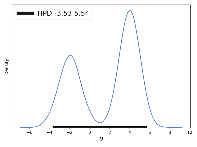
前文主要讨论的是对于单峰分布的概率分布求近似的HPD，但是对于双峰分布求解HPD并不是很好，如下图（前文内容中的图）：

 

 

 

 

 

 

==============================================================

 

 

 

 

我们求解的近似HPD中间有一个概率密度很低的区间，当然如果HPD可以不是一个连续区间的话我们可以有更好的求解方法呢，下面给出解法：

from __future__ import division
import matplotlib.pyplot as plt
import numpy as np
from scipy import stats
import seaborn as sns
palette = 'muted'
sns.set_palette(palette); sns.set_color_codes(palette)

np.random.seed(1)
gauss_a = stats.norm.rvs(loc=4, scale=0.9, size=3000)
gauss_b = stats.norm.rvs(loc=-2, scale=1, size=2000)
mix_norm = np.concatenate((gauss_a, gauss_b))





import numpy as np
import scipy.stats.kde as kde

def hpd_grid(sample, alpha=0.05, roundto=2):
    """Calculate highest posterior density (HPD) of array for given alpha.
    The HPD is the minimum width Bayesian credible interval (BCI).
    The function works for multimodal distributions, returning more than one mode

    Parameters
    ----------

    sample : Numpy array or python list
        An array containing MCMC samples
    alpha : float
        Desired probability of type I error (defaults to 0.05)
    roundto: integer
        Number of digits after the decimal point for the results

    Returns
    ----------
    hpd: array with the lower

    """
    sample = np.asarray(sample)
    sample = sample[~np.isnan(sample)]
    # get upper and lower bounds
    l = np.min(sample)
    u = np.max(sample)
    density = kde.gaussian_kde(sample)
    x = np.linspace(l, u, 2000)
    y = density.evaluate(x)
    # y = density.evaluate(x, l, u) waitting for PR to be accepted
    xy_zipped = zip(x, y / np.sum(y))
    xy = sorted(xy_zipped, key=lambda x: x[1], reverse=True)
    xy_cum_sum = 0
    hdv = []
    for val in xy:
        xy_cum_sum += val[1]
        hdv.append(val[0])
        if xy_cum_sum >= (1 - alpha):
            break
    hdv.sort()
    diff = (u - l) / 20  # differences of 5%
    hpd = []
    hpd.append(round(min(hdv), roundto))
    for i in range(1, len(hdv)):
        if hdv[i] - hdv[i - 1] >= diff:
            hpd.append(round(hdv[i - 1], roundto))
            hpd.append(round(hdv[i], roundto))
    hpd.append(round(max(hdv), roundto))
    ite = iter(hpd)
    hpd = list(zip(ite, ite))
    modes = []
    for value in hpd:
        x_hpd = x[(x > value[0]) & (x < value[1])]
        y_hpd = y[(x > value[0]) & (x < value[1])]
        modes.append(round(x_hpd[np.argmax(y_hpd)], roundto))
    return hpd, x, y, modes





import numpy as np
from scipy import stats
import matplotlib.pyplot as plt

def plot_post(sample, alpha=0.05, show_mode=True, kde_plot=True, bins=50,
              ROPE=None, comp_val=None, roundto=2):
    """Plot posterior and HPD

    Parameters
    ----------

    sample : Numpy array or python list
        An array containing MCMC samples
    alpha : float
        Desired probability of type I error (defaults to 0.05)
    show_mode: Bool
        If True the legend will show the mode(s) value(s), if false the mean(s)
        will be displayed
    kde_plot: Bool
        If True the posterior will be displayed using a Kernel Density Estimation
        otherwise an histogram will be used
    bins: integer
        Number of bins used for the histogram, only works when kde_plot is False
    ROPE: list or numpy array
        Lower and upper values of the Region Of Practical Equivalence
    comp_val: float
        Comparison value


    Returns
    -------

    post_summary : dictionary
        Containing values with several summary statistics

    """

    post_summary = {'mean': 0, 'median': 0, 'mode': 0, 'alpha': 0, 'hpd_low': 0,
                    'hpd_high': 0, 'comp_val': 0, 'pc_gt_comp_val': 0, 'ROPE_low': 0,
                    'ROPE_high': 0, 'pc_in_ROPE': 0}

    post_summary['mean'] = round(np.mean(sample), roundto)
    post_summary['median'] = round(np.median(sample), roundto)
    post_summary['alpha'] = alpha

    # Compute the hpd, KDE and mode for the posterior
    hpd, x, y, modes = hpd_grid(sample, alpha, roundto)
    post_summary['hpd'] = hpd
    post_summary['mode'] = modes

    ## Plot KDE.
    if kde_plot:
        plt.plot(x, y, color='k', lw=2)
    ## Plot histogram.
    else:
        plt.hist(sample, bins=bins, facecolor='b',
                 edgecolor='w')

    ## Display mode or mean:
    if show_mode:
        string = '{:g} ' * len(post_summary['mode'])
        plt.plot(0, label='mode =' + string.format(*post_summary['mode']), alpha=0)
    else:
        plt.plot(0, label='mean = {:g}'.format(post_summary['mean']), alpha=0)

    ## Display the hpd.
    hpd_label = ''
    for value in hpd:
        plt.plot(value, [0, 0], linewidth=10, color='b')
        hpd_label = hpd_label + '{:g} {:g}\n'.format(round(value[0], roundto), round(value[1], roundto))
    plt.plot(0, 0, linewidth=4, color='b', label='hpd {:g}%\n{}'.format((1 - alpha) * 100, hpd_label))
    ## Display the ROPE.
    if ROPE is not None:
        pc_in_ROPE = round(np.sum((sample > ROPE[0]) & (sample < ROPE[1])) / len(sample) * 100, roundto)
        plt.plot(ROPE, [0, 0], linewidth=20, color='r', alpha=0.75)
        plt.plot(0, 0, linewidth=4, color='r', label='{:g}% in ROPE'.format(pc_in_ROPE))
        post_summary['ROPE_low'] = ROPE[0]
        post_summary['ROPE_high'] = ROPE[1]
        post_summary['pc_in_ROPE'] = pc_in_ROPE
    ## Display the comparison value.
    if comp_val is not None:
        pc_gt_comp_val = round(100 * np.sum(sample > comp_val) / len(sample), roundto)
        pc_lt_comp_val = round(100 - pc_gt_comp_val, roundto)
        plt.axvline(comp_val, ymax=.75, color='g', linewidth=4, alpha=0.75,
                    label='{:g}% < {:g} < {:g}%'.format(pc_lt_comp_val,
                                                        comp_val, pc_gt_comp_val))
        post_summary['comp_val'] = comp_val
        post_summary['pc_gt_comp_val'] = pc_gt_comp_val

    plt.legend(loc=0, framealpha=1)
    frame = plt.gca()
    frame.axes.get_yaxis().set_ticks([])
    return post_summary


plot_post(mix_norm, roundto=2, alpha=0.05)
plt.legend(loc=0, fontsize=16)
plt.xlabel(r"$\theta$", fontsize=14)
plt.savefig('B04958_01_09.png', dpi=300, figsize=(5.5, 5.5))

plt.show()

 

这个代码的代码量比较大，其实功能和前文的逻辑是一致的。

 

对HPD区间的求解核心代码：

def hpd_grid(sample, alpha=0.05, roundto=2):
    """Calculate highest posterior density (HPD) of array for given alpha.
    The HPD is the minimum width Bayesian credible interval (BCI).
    The function works for multimodal distributions, returning more than one mode

    Parameters
    ----------

    sample : Numpy array or python list
        An array containing MCMC samples
    alpha : float
        Desired probability of type I error (defaults to 0.05)
    roundto: integer
        Number of digits after the decimal point for the results

    Returns
    ----------
    hpd: array with the lower

    """
    sample = np.asarray(sample)
    sample = sample[~np.isnan(sample)]
    # get upper and lower bounds
    l = np.min(sample)
    u = np.max(sample)
    density = kde.gaussian_kde(sample)
    x = np.linspace(l, u, 2000)
    y = density.evaluate(x)
    # y = density.evaluate(x, l, u) waitting for PR to be accepted
    xy_zipped = zip(x, y / np.sum(y))
    xy = sorted(xy_zipped, key=lambda x: x[1], reverse=True)
    xy_cum_sum = 0
    hdv = []
    for val in xy:
        xy_cum_sum += val[1]
        hdv.append(val[0])
        if xy_cum_sum >= (1 - alpha):
            break
    hdv.sort()
    diff = (u - l) / 20  # differences of 5%
    hpd = []
    hpd.append(round(min(hdv), roundto))
    for i in range(1, len(hdv)):
        if hdv[i] - hdv[i - 1] >= diff:
            hpd.append(round(hdv[i - 1], roundto))
            hpd.append(round(hdv[i], roundto))
    hpd.append(round(max(hdv), roundto))
    ite = iter(hpd)
    hpd = list(zip(ite, ite))
    modes = []
    for value in hpd:
        x_hpd = x[(x > value[0]) & (x < value[1])]
        y_hpd = y[(x > value[0]) & (x < value[1])]
        modes.append(round(x_hpd[np.argmax(y_hpd)], roundto))
    return hpd, x, y, modes

 

同样都是使用蒙特卡洛模拟方法，但是与前文内容这里并不是直接使用原始概率分布来生成采样数据（似然分布）而是将获得的原始分布的数据进行高斯核函数估计出一个概率密度（概率函数），然后用这个估计出的概率函数再重新生成数据，这种方法虽然会造成得到的概率分布和原始概率分布的一定偏差不过该种方法十分适合无法获得原始概率分布的情况，而且经过本人测试使用高斯核函数估计出的概率函数基本和原始的概率分布吻合（十分的神奇）。

 

生成新的概率分布函数：

density = kde.gaussian_kde(sample)

 

生成新的样本数据：

    x = np.linspace(l, u, 2000)
    y = density.evaluate(x)

 

对新生成的样本数据数据的对应概率密度进行规则化：（ 这样可以保证即使采样的数据量不是十分大的情况下生成的数据对应的概率密度区间的面积和为1，方便下面对0.95HPD区间面积加和求解时的计算）

xy_zipped = zip(x, y / np.sum(y))

 

 

对0.95的HPD区间求解，原理就是将区间各点概率从大到小排序然后求得加总后等于0.95的最少的区间点，这也是上一步对各点概率进行规则化的主要原因。这步求得的点对应的概率加和为0.95，并且保证样本点数目最少，这样也保证对应的区间尽可能的小以满足近似HPD最小区间的要求。

    xy = sorted(xy_zipped, key=lambda x: x[1], reverse=True)
    xy_cum_sum = 0
    hdv = []
    for val in xy:
        xy_cum_sum += val[1]
        hdv.append(val[0])
        if xy_cum_sum >= (1 - alpha):
            break
    hdv.sort()

 

 

 

 

 

 

设置一个区间阈值diff，如果上一步求得的区间中如果有两个排序后相邻的点之间距离大于这个阈值就认为这两个点是不连续的（分属两个区间中），然后记录这两个点。计算结束后记录上步求得的HPD区间中的两个边界点。这样求得的hpd列表中每两个数代表一个区间，这样就保证最后求得的HPD区间可以是不连续的。

    diff = (u - l) / 20  # differences of 5%
    hpd = []
    hpd.append(round(min(hdv), roundto))
    for i in range(1, len(hdv)):
        if hdv[i] - hdv[i - 1] >= diff:
            hpd.append(round(hdv[i - 1], roundto))
            hpd.append(round(hdv[i], roundto))
    hpd.append(round(max(hdv), roundto))

这一步中求得的hpd列表为[-4.06, 0.16, 1.82, 6.18]，其中[-4.06, 0.16,]代表一个区间，[1.82, 6.18]代表另一个区间。

 

 

 

 

 

上面的核心代码中还有求解所谓的众数的代码，由于这个概率分布时连续的因此所谓的众数就是概率密度最大的数。

ite = iter(hpd)
hpd = list(zip(ite, ite))
modes = []
for value in hpd:
    x_hpd = x[(x > value[0]) & (x < value[1])]
    y_hpd = y[(x > value[0]) & (x < value[1])]
    modes.append(round(x_hpd[np.argmax(y_hpd)], roundto))
return hpd, x, y, modes

上面的代码不难，不过有个很有意思的python代码，其实搞python代码快10多个年头了即使是今天还会遇到一些没发现过的pythonic的代码，上面就有这种：

 

 

 

 

 

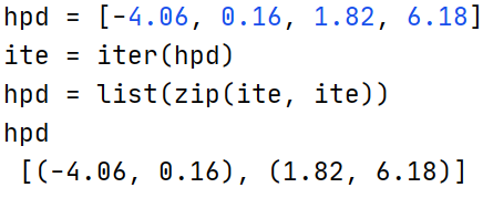
ite为列表hpd的迭代器。

zip(ite,ite)是惰性计算，在list(zip(ite,ite))时才会从迭代器ite中提取数据，虽然zip每次从两个迭代器中提取数据但是这两个迭代器都是一个ite迭代器，那么就会zip每次从两个ite中提取数据实际都是一个ite提供的，因此最终的提取结果就是hpd中的数据依次提取两个，最后的提取结果就是[(-4.06, 0.16), (1.82, 6.18)]。如果不这样写可能就得这么写这个代码了：

hpd2=[ ]

for i in range(1, len(hpd)):

    hpd2.append((hpd[i-1], hpd[i]))

print(hpd2)

 

 

 

 

 

 

=========================================================