

9日笔记
今天很累 注个水 到15日再整理博客,把错的,虚假的题解删除(一批)
ML week 1 和 week 2 和 week3
Python代码实现,带注解的ipynb 【黄广博版】 复现 原理理解和头脑里推一边**------------恢复内容开始------------*
如若引用请到github找fengdu78
Chapter2. logistic_regression(逻辑回归)
① 准备数据
sns.set(context="notebook", style="darkgrid", palette=sns.color_palette("RdBu", 2))

sns.lmplot('exam1', 'exam2', hue='admitted', data=data,
           size=6,
           fit_reg=False,
           scatter_kws={"s": 50}
          )
plt.show()#看下数据的样子
def get_X(df):#读取特征
#     """
#     use concat to add intersect feature to avoid side effect
#     not efficient for big dataset though
#     """
    ones = pd.DataFrame({'ones': np.ones(len(df))})#ones是m行1列的dataframe
    data = pd.concat([ones, df], axis=1)  # 合并数据,根据列合并
    return data.iloc[:, :-1].as_matrix()  # 这个操作返回 ndarray,不是矩阵
def get_y(df):#读取标签
#     '''assume the last column is the target'''
    return np.array(df.iloc[:, -1])#df.iloc[:, -1]是指df的最后一列
def normalize_feature(df):
#     """Applies function along input axis(default 0) of DataFrame."""
    return df.apply(lambda column: (column - column.mean()) / column.std())#特征缩放
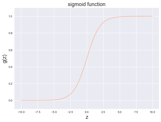
sigmoid 函数
g 代表一个常用的逻辑函数(logistic function)为S形函数(Sigmoid function),公式为:\[g\left( z \right)=\frac{1}{1+{{e}^{-z}}}\]
合起来,我们得到逻辑回归模型的假设函数:
\[{{h}_{\theta }}\left( x \right)=\frac{1}{1+{{e}^{-{{\theta }^{T}}X}}}\]
代码:
def sigmoid(z):
    return 1 / (1 + np.exp(-z))
In [11]:
fig, ax = plt.subplots(figsize=(8, 6))
ax.plot(np.arange(-10, 10, step=0.01),
        sigmoid(np.arange(-10, 10, step=0.01)))
ax.set_ylim((-0.1,1.1))
ax.set_xlabel('z', fontsize=18)
ax.set_ylabel('g(z)', fontsize=18)
ax.set_title('sigmoid function', fontsize=18)
plt.show()
cost function(代价函数)
- \(max(\ell(\theta)) = min(-\ell(\theta))\)
- choose \(-\ell(\theta)\) as the cost function
\[\begin{align}
& J\left( \theta \right)=-\frac{1}{m}\sum\limits_{i=1}^{m}{[{{y}^{(i)}}\log \left( {{h}_{\theta }}\left( {{x}^{(i)}} \right) \right)+\left( 1-{{y}^{(i)}} \right)\log \left( 1-{{h}_{\theta }}\left( {{x}^{(i)}} \right) \right)]} \\
& =\frac{1}{m}\sum\limits_{i=1}^{m}{[-{{y}^{(i)}}\log \left( {{h}_{\theta }}\left( {{x}^{(i)}} \right) \right)-\left( 1-{{y}^{(i)}} \right)\log \left( 1-{{h}_{\theta }}\left( {{x}^{(i)}} \right) \right)]} \\
\end{align}\]
gradient descent(梯度下降)
- 这是批量梯度下降(batch gradient descent)
- 转化为向量化计算: \(\frac{1}{m} X^T( Sigmoid(X\theta) - y )\)
\[\frac{\partial J\left( \theta \right)}{\partial {{\theta }_{j}}}=\frac{1}{m}\sum\limits_{i=1}^{m}{({{h}_{\theta }}\left( {{x}^{(i)}} \right)-{{y}^{(i)}})x_{_{j}}^{(i)}}
\]
拟合参数
- 这里我使用
scipy.optimize.minimize去寻找参数
import scipy.optimize as opt
res = opt.minimize(fun=cost, x0=theta, args=(X, y), method='Newton-CG', jac=gradient)
print(res)
用训练集预测和验证
def predict(x, theta):
    prob = sigmoid(x @ theta)
    return (prob >= 0.5).astype(int)

final_theta = res.x
y_pred = predict(X, final_theta)

print(classification_report(y, y_pred))
| precision | recall | f1-score | support | |
|---|---|---|---|---|
| 0 | 0.87 | 0.85 | 0.86 | 40 |
| 1 | 0.90 | 0.92 | 0.91 | 60 |
| avg / total | 0.89 | 0.89 | 0.89 | 100 |
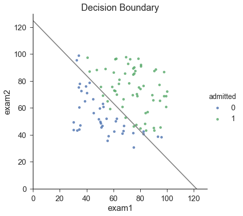
寻找决策边界
\(X \times \theta = 0\) (this is the line)
print(res.x) # this is final theta
[-25.16227358 0.20623923 0.20147921]
coef = -(res.x / res.x[2])  # find the equation
print(coef)

x = np.arange(130, step=0.1)
y = coef[0] + coef[1]*x
[ 124.88769463 -1.0236254 -1. ]
data.describe() # find the range of x and y
| exam1 | exam2 | admitted | |
|---|---|---|---|
| count | 100.000000 | 100.000000 | 100.000000 |
| mean | 65.644274 | 66.221998 | 0.600000 |
| std | 19.458222 | 18.582783 | 0.492366 |
| min | 30.058822 | 30.603263 | 0.000000 |
| 25% | 50.919511 | 48.179205 | 0.000000 |
| 50% | 67.032988 | 67.682381 | 1.000000 |
| 75% | 80.212529 | 79.360605 | 1.000000 |
| max | 99.827858 | 98.869436 | 1.000000 |
截距(与y轴交点)大概会在125 对x/y. you know the intercept would be around 125 for both x and y
------------恢复内容结束------------
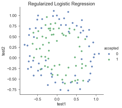
3- 正则化逻辑回归
df = pd.read_csv('ex2data2.txt', names=['test1', 'test2', 'accepted'])
df.head()
sns.set(context="notebook", style="ticks", font_scale=1.5)

sns.lmplot('test1', 'test2', hue='accepted', data=df,
           size=6,
           fit_reg=False,
           scatter_kws={"s": 50}
          )

plt.title('Regularized Logistic Regression')
plt.show()
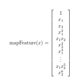
feature mapping(特征映射)
for i in 0..i
  for p in 0..i:
    output x^(i-p) * y^p
def feature_mapping(x, y, power, as_ndarray=False):
#     """return mapped features as ndarray or dataframe"""
    # data = {}
    # # inclusive
    # for i in np.arange(power + 1):
    #     for p in np.arange(i + 1):
    #         data["f{}{}".format(i - p, p)] = np.power(x, i - p) * np.power(y, p)

    data = {"f{}{}".format(i - p, p): np.power(x, i - p) * np.power(y, p)
                for i in np.arange(power + 1)
                for p in np.arange(i + 1)
            }

    if as_ndarray:
        return pd.DataFrame(data).as_matrix()
    else:
        return pd.DataFrame(data)
In [34]:
x1 = np.array(df.test1)
x2 = np.array(df.test2)
In [35]:
data = feature_mapping(x1, x2, power=6)
print(data.shape)
data.head()
data.describe()
regularized cost(正则化代价函数)
\[J\left( \theta \right)=\frac{1}{m}\sum\limits_{i=1}^{m}{[-{{y}^{(i)}}\log \left( {{h}_{\theta }}\left( {{x}^{(i)}} \right) \right)-\left( 1-{{y}^{(i)}} \right)\log \left( 1-{{h}_{\theta }}\left( {{x}^{(i)}} \right) \right)]}+\frac{\lambda }{2m}\sum\limits_{j=1}^{n}{\theta _{j}^{2}}
\]
def regularized_cost(theta, X, y, l=1):
#     '''you don't penalize theta_0'''
    theta_j1_to_n = theta[1:]
    regularized_term = (l / (2 * len(X))) * np.power(theta_j1_to_n, 2).sum()

    return cost(theta, X, y) + regularized_term
#正则化代价函数
regularized gradient(正则化梯度)
\[\frac{\partial J\left( \theta \right)}{\partial {{\theta }_{j}}}=\left( \frac{1}{m}\sum\limits_{i=1}^{m}{\left( {{h}_{\theta }}\left( {{x}^{\left( i \right)}} \right)-{{y}^{\left( i \right)}} \right)} \right)+\frac{\lambda }{m}{{\theta }_{j}}\text{ }\text{ for j}\ge \text{1}
\]
def regularized_gradient(theta, X, y, l=1):
#     '''still, leave theta_0 alone'''
    theta_j1_to_n = theta[1:]
    regularized_theta = (l / len(X)) * theta_j1_to_n

    # by doing this, no offset is on theta_0
    regularized_term = np.concatenate([np.array([0]), regularized_theta])

    return gradient(theta, X, y) + regularized_term
拟合参数
import scipy.optimize as opt
In [47]:
print('init cost = {}'.format(regularized_cost(theta, X, y)))

res = opt.minimize(fun=regularized_cost, x0=theta, args=(X, y), method='Newton-CG', jac=regularized_gradient)
res
预测
In [48]:
final_theta = res.x
y_pred = predict(X, final_theta)

print(classification_report(y, y_pred))
| precision | recall | f1-score | support | |
|---|---|---|---|---|
| 0 | 0.90 | 0.75 | 0.82 | 60 |
| 1 | 0.78 | 0.91 | 0.84 | 58 |
| avg / total | 0.84 | 0.83 | 0.83 | 118 |
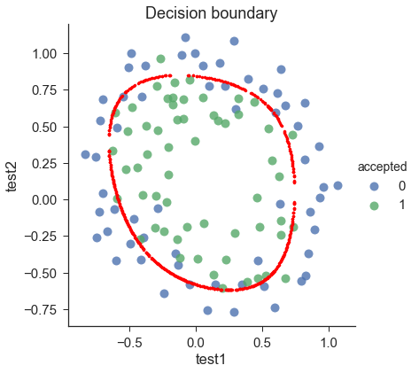
使用不同的 \(\lambda\) (这个是常数)画出决策边界
- 我们找到所有满足 \(X\times \theta = 0\) 的x
- instead of solving polynomial equation, just create a coridate x,y grid that is dense enough, and find all those \(X\times \theta\) that is close enough to 0, then plot them
def draw_boundary(power, l):
#     """
#     power: polynomial power for mapped feature
#     l: lambda constant
#     """
    density = 1000
    threshhold = 2 * 10**-3

    final_theta = feature_mapped_logistic_regression(power, l)
    x, y = find_decision_boundary(density, power, final_theta, threshhold)

    df = pd.read_csv('ex2data2.txt', names=['test1', 'test2', 'accepted'])
    sns.lmplot('test1', 'test2', hue='accepted', data=df, size=6, fit_reg=False, scatter_kws={"s": 100})

    plt.scatter(x, y, c='R', s=10)
    plt.title('Decision boundary')
    plt.show()
def feature_mapped_logistic_regression(power, l):
#     """for drawing purpose only.. not a well generealize logistic regression
#     power: int
#         raise x1, x2 to polynomial power
#     l: int
#         lambda constant for regularization term
#     """
    df = pd.read_csv('ex2data2.txt', names=['test1', 'test2', 'accepted'])
    x1 = np.array(df.test1)
    x2 = np.array(df.test2)
    y = get_y(df)

    X = feature_mapping(x1, x2, power, as_ndarray=True)
    theta = np.zeros(X.shape[1])

    res = opt.minimize(fun=regularized_cost,
                       x0=theta,
                       args=(X, y, l),
                       method='TNC',
                       jac=regularized_gradient)
    final_theta = res.x

    return final_theta
def find_decision_boundary(density, power, theta, threshhold):
    t1 = np.linspace(-1, 1.5, density)
    t2 = np.linspace(-1, 1.5, density)

    cordinates = [(x, y) for x in t1 for y in t2]
    x_cord, y_cord = zip(*cordinates)
    mapped_cord = feature_mapping(x_cord, y_cord, power)  # this is a dataframe

    inner_product = mapped_cord.as_matrix() @ theta

    decision = mapped_cord[np.abs(inner_product) < threshhold]

    return decision.f10, decision.f01
#寻找决策边界函数
draw_boundary(power=6, l=1)#lambda=1
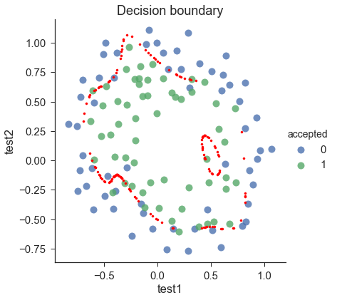
draw_boundary(power=6, l=0) # no regularization, over fitting,#lambda=0,没有正则化,过拟合了
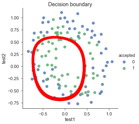
draw_boundary(power=6, l=100) # underfitting,#lambda=100,欠拟合

 浙公网安备 33010602011771号