import pandas as pd
import numpy as np
import matplotlib.pyplot as plt
import seaborn as sns
import sys
from GM11 import GM11
inputfile = '../data/data.csv' # 输出的数据文件
data = pd.read_csv(inputfile) # 读数据
# 对各属性进行描述性统计分析
def statisticAnalysis(data):
# 最小值、最大值、均值、标准差
description = [data.min(), data.max(), data.mean(), data.std()]
# 将结果存入数据框
description = pd.DataFrame(description, index=["Min", "Max", "Mean", "STD"]).T
print("描述性统计结果:\n", np.round(description, 2)) # 保留两位
# 求解原始数据的Pearson相关系数矩阵
def correlationCoefficientMatrix(data):
corr = data.corr(method='pearson') # 计算相关系数矩阵
print("相关系数矩阵为:\n", np.round(corr, 2)) # 保留两位
return corr
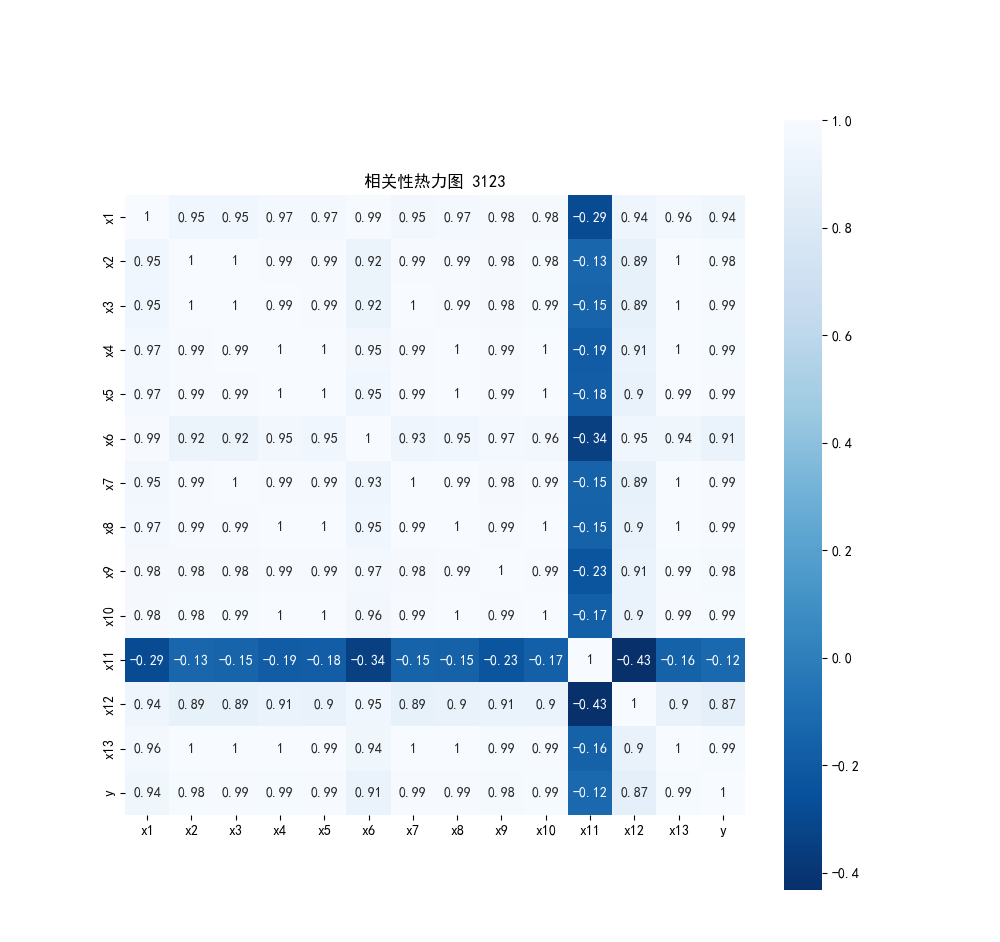
# 绘制相关性热力图
def thermodynamic(corr):
plt.rcParams['font.sans-serif'] = ['SimHei'] # 显示中文标签
plt.rcParams['axes.unicode_minus']=False
plt.subplots(figsize=(10, 10))
sns.heatmap(corr, annot=True, vmax=1, square=True, cmap="Blues_r")
plt.title("相关性热力图 3123")
plt.show()
plt.close()
# 构建灰色预测模型并预测
def grey():
sys.path.append("D:/作业/数据挖掘/tmp")
inputfile1 = "../data/new_reg_data.csv"
inputfile2 = "../data/data.csv"
new_reg_data = pd.read_csv(inputfile1)
data = pd.read_csv(inputfile2)
new_reg_data.index = range(1994, 2014)
new_reg_data.loc[2014] = None
new_reg_data.loc[2015] = None
cols = ['x1', 'x3', 'x4', 'x5', 'x6', 'x7', 'x8', 'x13']
for i in cols:
f = GM11(new_reg_data.loc[range(1994, 2014), i].values)[0]
new_reg_data.loc[2014, i] = f(len(new_reg_data)-1) # 2014年预测结果
new_reg_data.loc[2015, i] = f(len(new_reg_data)) # 2015年预测结果
new_reg_data[i] = new_reg_data[i].round(2)
outputfile = '../tmp/new_reg_data_GM11.xls' # 灰色预测后保存路径
y = list(data['y'].values)
y.extend([np.nan, np.nan])
new_reg_data['y'] = y
new_reg_data.to_excel(outputfile)
print("预测结果为:\n",new_reg_data.loc[2014:2015,:])
# 构建支持向量回归预测模型
def SVR():
from sklearn.svm import LinearSVR
inputfile = '../tmp/new_reg_data_GM11.xls'
data = pd.read_excel(inputfile)
feature = ['x1', 'x3', 'x4', 'x5', 'x6', 'x7', 'x8', 'x13']
data.index = range(1994, 2016)
data_train = data.loc[range(1994, 2014)].copy()
data_mean = data_train.mean()
data_std = data_train.std()
data_train = (data_train - data_mean)/data_std
x_train = data_train[feature].to_numpy()
y_train = data_train['y'].to_numpy()
linearsvr = LinearSVR()
linearsvr.fit(x_train, y_train)
x = ((data[feature] - data_mean[feature])/data_std[feature]).to_numpy()
data[u'y_pred'] = linearsvr.predict(x) * data_std['y'] + data_mean['y']
# outputfile = '../tmp/new_reg_data_GM11_revenue.xls'
# data.to_excel(outputfile)
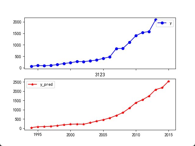
print("真实值与预测值分别为:\n",data[['y', 'y_pred']])
plt.rcParams['font.sans-serif'] = ['SimHei'] # 显示中文标签
plt.rcParams['axes.unicode_minus'] = False
fig = data[['y', 'y_pred']].plot(subplots = True,style=['b-o', 'r-*'])
plt.title("3123")
plt.show()
statisticAnalysis(data)
corr = correlationCoefficientMatrix(data)
thermodynamic(corr)
grey()
SVR()


 浙公网安备 33010602011771号