tensorflow2.0——鸢尾花数据集的一元分类

import tensorflow as tf
import numpy as np
import pandas as pd
import matplotlib.pylab as plt
import matplotlib as mpl

#   读取数据集
TRIN_URL = 'http://download.tensorflow.org/data/iris_training.csv'            # 数据集下载网址
df_iris = pd.read_csv('./鸢尾花数据集/iris.csv', header=0)                   # 读取本地csv文件数据
df_iris_test = pd.read_csv('./鸢尾花数据集/iris_test.csv', header=0)
# print(df_iris)                                                              #   最后一列是分类编号
#   处理数据集
iris = np.array(df_iris)                                                        # 将数据转换成numpy数组
iris_test = np.array(df_iris_test)
iris2 = iris[iris[:, -1] < 2]                                                   # 只取分类编号小于2的两类数据
iris2_test = iris_test[iris_test[:, -1] < 2]
#   训练集数据处理
train_x = iris2[:, 0:2]                                                         # 只取特征的前两列
train_x = train_x - np.mean(train_x, axis=0)                                     # 需要将样本的均值变为0
train_1 = np.ones(train_x.shape[0]).reshape(-1, 1)                               # 生成一个与train_x一样行数的全1矩阵
# print('train_1:',train_1)
train_x = tf.concat((train_x, train_1), axis=1)                                  # 将train_x扩充一列全1
train_x = tf.cast(train_x,tf.float32)
#   测试集遵循上面训练集的操作
test_x = iris2_test[:, 0:2]
test_x = test_x - np.mean(test_x, axis=0)
test_1 = np.ones(test_x.shape[0]).reshape(-1, 1)
test_x = tf.concat((test_x, test_1), axis=1)
test_x = tf.cast(test_x,tf.float32)

train_y = iris2[:, -1]  # 标签
train_y = train_y.reshape(-1,1)
test_y = iris2_test[:, -1]  # 标签
test_y = test_y.reshape(-1,1)
# print('axis = 0:',np.mean(train_x,axis=0))                                    #   axis = 0 求一列的平均值
# print(train_y, train_y.shape)
print(test_y, test_y.shape)

#   设置超参
iter = 2000
learn_rate = 0.1
loss_list = []
acc_list = []
#   初始化训练参数

w = tf.Variable(np.random.randn(3,1),dtype=tf.float32)
# w = tf.Variable(np.array([1.,1.,1.]).reshape(-1,1),dtype=tf.float32)

for i in range(iter):
    with tf.GradientTape() as tape:
        y_p = 1 / (1 + tf.exp(-(tf.matmul(train_x, w))))
        loss = tf.reduce_mean(-(train_y * tf.math.log(y_p) + (1 - train_y) * tf.math.log(1 - y_p)))
    dloss_dw = tape.gradient(loss, w)
    w.assign_sub(learn_rate * dloss_dw)
    loss_list.append(loss)
    acc = tf.reduce_mean(tf.cast(tf.equal(tf.round(y_p),train_y),dtype = tf.float32))
    acc_list.append(acc)
    if i % 100 == 0:
        print('第{}次, loss:{},acc:{}'.format(i,loss,acc))
        # print('y_p:{}\ntrain_y:{}'.format(y_p, train_y))
        print()


#   预测直线的横纵坐标处理
    #   训练集
x1 = train_x[:,0]
print(w[0] * 55)
x2 = -(w[0] * x1 + w[2])/ w[1]
# print('x2:',x2)
    #   测试集
x1_test = test_x[:,0]
print(w[0] * 55)
x2_test = -(w[0] * x1_test + w[2])/ w[1]

#   画图
plt.rcParams["font.family"] = 'SimHei'                          # 将字体改为中文
plt.rcParams['axes.unicode_minus'] = False                      # 设置了中文字体默认后，坐标的"-"号无法显示，设置这个参数就可以避免
#   分子图开始画图
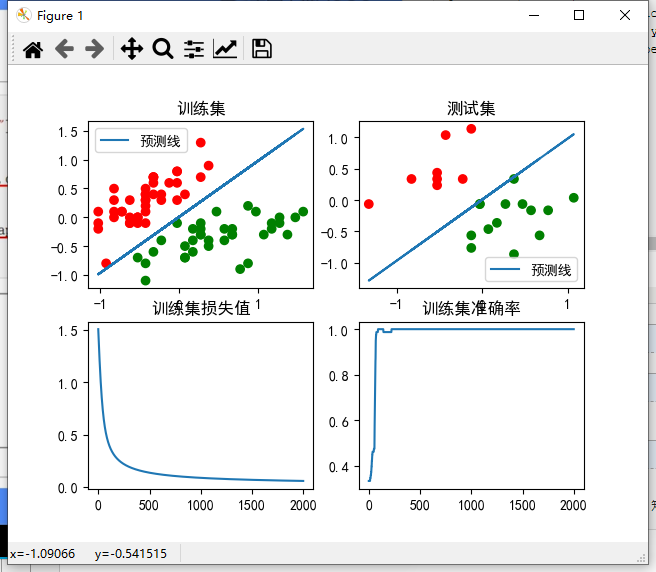
plt.subplot(221)
plt.title('训练集')
cm_pt = mpl.colors.ListedColormap(['red', 'green'])
plt.scatter(x=train_x[:, 0], y=train_x[:, 1], c=train_y, cmap=cm_pt)
plt.plot(x1,x2,label = '预测线')
plt.legend()

plt.subplot(222)
plt.title('测试集')
cm_pt = mpl.colors.ListedColormap(['red', 'green'])
plt.scatter(x=test_x[:, 0], y=test_x[:, 1], c=test_y, cmap=cm_pt)
plt.plot(x1_test,x2_test,label = '预测线')
plt.legend()

plt.subplot(223)
plt.title('训练集损失值')
plt.plot(loss_list)
plt.subplot(224)
plt.title('训练集准确率')
plt.plot(acc_list)
plt.show()