
记录一次简单模型训练的结果-04
代码:
点击查看代码
"""
Created on Tue Feb 11 15:34:18 2025
blog: https://www.cnblogs.com/cs1study
@author: cs1study
"""
# 3.数据清洗与预处理
from sklearn.datasets import fetch_california_housing
import pandas as pd
# 加载 California Housing 数据集
housing = fetch_california_housing()
data = pd.DataFrame(housing.data, columns=housing.feature_names)
data['PRICE'] = housing.target
print(data.isnull().sum())
from sklearn.preprocessing import StandardScaler
# 特征标准化
scaler = StandardScaler()
features = data.drop('PRICE', axis=1)
target = data['PRICE']
features_scaled = scaler.fit_transform(features)
# 4.训练一个简单模型
from sklearn.model_selection import train_test_split
# 划分训练集和测试集
X_train, X_test, y_train, y_test = train_test_split(features_scaled, target, test_size=0.2, random_state=42)
from sklearn.linear_model import LinearRegression
from sklearn.metrics import mean_squared_error, r2_score
# 初始化模型
model = LinearRegression()
# 训练模型
model.fit(X_train, y_train)
# 预测
y_pred = model.predict(X_test)
# 评估性能
mse = mean_squared_error(y_test, y_pred)
r2 = r2_score(y_test, y_pred)
print(f"均方误差(MSE):{mse}")
print(f"R2 分数:{r2}")
# 5构建一个简单神经网络
from tensorflow.keras.models import Sequential
from tensorflow.keras.layers import Dense, Dropout, Input
from tensorflow.keras.optimizers import Adam
# 构建更深的神经网络
nn_model = Sequential([
Input(shape=(X_train.shape[1],)), # 使用 Input 层显式定义输入形状
Dense(256, activation='relu'), # 第一隐藏层,256个神经元
Dense(128, activation='relu'), # 第二隐藏层
Dense(64, activation='relu'), # 第三隐藏层
Dense(1) # 输出层
])
# 编译模型
nn_model.compile(optimizer=Adam(learning_rate=0.0001), loss='mse', metrics=['mae'])
# 训练模型
history = nn_model.fit(
X_train, y_train,
epochs=200, # 增加训练轮数
batch_size=64, # 调整批量大小
validation_split=0.2, # 20%数据用于验证
verbose=1 # 显示训练过程
)
'''
# 监控训练过程
from tensorflow.keras.callbacks import EarlyStopping
# 添加早停法
early_stop = EarlyStopping(monitor='val_loss', patience=10, restore_best_weights=True)
# 设置 patience 参数,允许验证损失在指定的轮次内未改善时终止训练
history = nn_model.fit(
X_train, y_train,
epochs=200,
batch_size=64,
validation_split=0.2,
callbacks=[early_stop] # 应用早停
)
'''
# 模型评估
test_loss, test_mae = nn_model.evaluate(X_test, y_test)
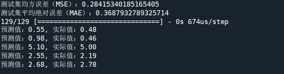
print(f"测试集均方误差(MSE):{test_loss}")
print(f"测试集平均绝对误差(MAE):{test_mae}")
# 用测试集数据预测
predictions = nn_model.predict(X_test)
# 显示部分预测结果
for i in range(5):
print(f"预测值:{predictions[i][0]:.2f}, 实际值:{y_test.iloc[i]:.2f}")
import matplotlib.pyplot as plt
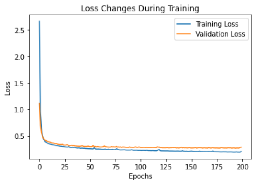
# 绘制训练和验证损失
plt.plot(history.history['loss'], label='Training Loss') # 训练损失
plt.plot(history.history['val_loss'], label='Validation Loss') # 验证损失
plt.xlabel('Epochs')
plt.ylabel('Loss')
plt.legend()
plt.title('Loss Changes During Training') # 训练过程中的损失变化
plt.show()
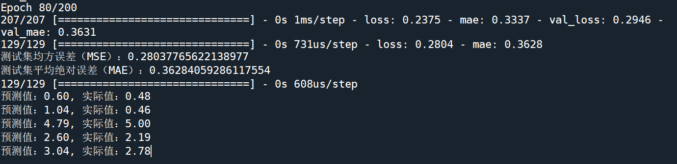
结果的截图:
这里对这个模型的200次训练进行了监控,只用80次就完成了训练。
代码:
点击查看代码
"""
Created on Tue Feb 11 15:34:18 2025
blog: https://www.cnblogs.com/cs1study
@author: cs1study
"""
# 3.数据清洗与预处理
from sklearn.datasets import fetch_california_housing
import pandas as pd
# 加载 California Housing 数据集
housing = fetch_california_housing()
data = pd.DataFrame(housing.data, columns=housing.feature_names)
data['PRICE'] = housing.target
print(data.isnull().sum())
from sklearn.preprocessing import StandardScaler
# 特征标准化
scaler = StandardScaler()
features = data.drop('PRICE', axis=1)
target = data['PRICE']
features_scaled = scaler.fit_transform(features)
# 4.训练一个简单模型
from sklearn.model_selection import train_test_split
# 划分训练集和测试集
X_train, X_test, y_train, y_test = train_test_split(features_scaled, target, test_size=0.2, random_state=42)
from sklearn.linear_model import LinearRegression
from sklearn.metrics import mean_squared_error, r2_score
# 初始化模型
model = LinearRegression()
# 训练模型
model.fit(X_train, y_train)
# 预测
y_pred = model.predict(X_test)
# 评估性能
mse = mean_squared_error(y_test, y_pred)
r2 = r2_score(y_test, y_pred)
print(f"均方误差(MSE):{mse}")
print(f"R2 分数:{r2}")
# 5构建一个简单神经网络
from tensorflow.keras.models import Sequential
from tensorflow.keras.layers import Dense, Dropout, Input
from tensorflow.keras.optimizers import Adam
# 构建更深的神经网络
nn_model = Sequential([
Input(shape=(X_train.shape[1],)), # 使用 Input 层显式定义输入形状
Dense(256, activation='relu'), # 第一隐藏层,256个神经元
Dense(128, activation='relu'), # 第二隐藏层
Dense(64, activation='relu'), # 第三隐藏层
Dense(1) # 输出层
])
# 编译模型
nn_model.compile(optimizer=Adam(learning_rate=0.0001), loss='mse', metrics=['mae'])
# 训练模型
'''
history = nn_model.fit(
X_train, y_train,
epochs=200, # 增加训练轮数
batch_size=64, # 调整批量大小
validation_split=0.2, # 20%数据用于验证
verbose=1 # 显示训练过程
)
'''
# 监控训练过程
from tensorflow.keras.callbacks import EarlyStopping
# 添加早停法
early_stop = EarlyStopping(monitor='val_loss', patience=10, restore_best_weights=True)
# 设置 patience 参数,允许验证损失在指定的轮次内未改善时终止训练
history = nn_model.fit(
X_train, y_train,
epochs=200,
batch_size=64,
validation_split=0.2,
callbacks=[early_stop] # 应用早停
)
# 模型评估
test_loss, test_mae = nn_model.evaluate(X_test, y_test)
print(f"测试集均方误差(MSE):{test_loss}")
print(f"测试集平均绝对误差(MAE):{test_mae}")
# 用测试集数据预测
predictions = nn_model.predict(X_test)
# 显示部分预测结果
for i in range(5):
print(f"预测值:{predictions[i][0]:.2f}, 实际值:{y_test.iloc[i]:.2f}")
import matplotlib.pyplot as plt
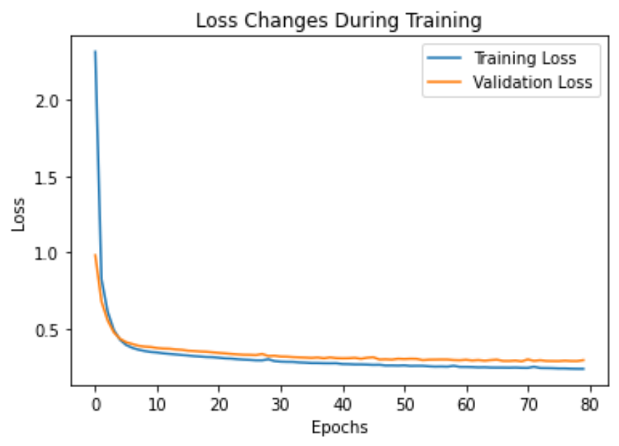
# 绘制训练和验证损失
plt.plot(history.history['loss'], label='Training Loss') # 训练损失
plt.plot(history.history['val_loss'], label='Validation Loss') # 验证损失
plt.xlabel('Epochs')
plt.ylabel('Loss')
plt.legend()
plt.title('Loss Changes During Training') # 训练过程中的损失变化
plt.show()
截图:

 浙公网安备 33010602011771号