R语言-数据类型、结构以及对象类型2

R数据类型与对象_转载

前言

  R函数只能接受指定数据类型的变量，否则函数不能执行,并报错。可以用is.*函数来判断函数是否属于某种类型，不同类型之间可以通过as.*来转换。

  R对象有如下的属性：

	names, dimnames 名字 维数的名字
	dimensions (e.g. matrices, arrays) 维度
	class 类别
	length 长度
	# 其他的一些用户定义的属性
	对象的属性可以用attributes()这个功能来知道

目录

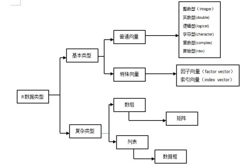
 1. 普通向量

 2. 特殊向量

 3. 复杂数据类型

 4. 部分常用的函数

1. 普通向量

  向量是相同类型的元素组成的有序集合，这个“序”体现为可以通过下表索引来访问集合中的元素。普通向量根据其元素的组成不同，可以分为上图6种。元素必须为同一类型的数据。

	> vector1<-c(0,1,2,1,-1) #构建向量vector
	> vector1 #查看向量内容 
	[1] 0 1 2 1 -1 
	> is.numeric(vector1) #判断是否为数字类型向量
	[1] TRUE
	> as.character(vector1) #转化为字符向量
	[1] "0" "1" "2" "1" "-1"
	> data.class(vector1)
	[1] "numeric"
	> vector1<-as.character(vector1) #转化为字符向量后写入vector1
	> data.class(vector1) #判断变量类型
	[1] "character"
	> as.logical(vector1)
	[1] NA NA NA NA NA
	> vector1<-as.numeric(vector1)
	> data.class(vector1)
	[1] "numeric"
	> as.logical(vector1) #只有0转化为FALSE
	[1] FALSE TRUE TRUE TRUE TRUE

  逻辑向量。0为假，其它为真。

	> a=0
	> as.logical(a)
	[1] FALSE
	> b=-1
	> as.logical(b)
	[1] TRUE
	> c=1
	> as.logical(c)
	[1] TRUE

  我们也可以通过as这个功能来调整向量的属性。

	> x <- 0:6
	> class(x)
	[1] "integer"
	> as.numeric(x)
	[1] 0 1 2 3 4 5 6
	> as.logical(x)
	[1] FALSE TRUE TRUE TRUE TRUE TRUE TRUE
	> as.character(x)
	[1] "0" "1" "2" "3" "4" "5" "6"
	> as.complex(x)
	[1] 0+0i 1+0i 2+0i 3+0i 4+0i 5+0i 6+0i

  向量的运算

	向量元素的循环使用（不同长度的向量的运算）
	x+y

2. 特殊向量

  特殊类型的向量包括因子向量与索引向量，他们的类型，模式和存储模式与整数向量一致。对因子向量进行分组，相同的归为一组，每组为一个Level,有点Unique的味道，相当于统计中的分类变量。因子向量分为有序与无序两种。它们在一些统计分析中起作用。

	> vector1<-c(0,1,2,1,-1)
	> vector1<-as.factor(vector1)
	> vector1
	[1] 0 1 2 1 -1
	Levels: -1 0 1 2
	> levels(vector1)
	[1] "-1" "0" "1" "2" 
	> vector1<-ordered(vector1)
	> vector1
	[1] 0 1 2 1 -1
	Levels: -1 < 0 < 1 < 2

  索引向量（index vector）
  也叫下表向量，它的主要作用就是数据选择。例如可以在向量名后面跟的方括号中加入索引向量以得到向量的子集。索引向量可以是整数向量，负整数向量，逻辑向量和字符串向量。

	> vector1<-c(0,1,2,1,-1)
	> vector1[2]
	[1] 1
	> vector1[2:4]
	[1] 1 2 1
	> vector1[-4] #不要第四个数
	[1] 0 1 2 -1
	> vector1[-(1:2)]
	[1] 2 1 -1
	> vector2<-c(0,1,2,NA,4,5,-1)
	> vector2[vector2>0]
	[1] 1 2 NA 4 5
	> vector2[!is.na(vector2)]
	[1] 0 1 2 4 5 -1
	> vector2[!is.na(vector2) & vector2>0] #&表示合的意思
	[1] 1 2 4 5

  因子（factor）向量

	因子是一个分类变量，用于描述分类数据。一般因子有多个水平（levels）.
	因子向量中元素类型必须相同
	创建一个因子
	factor()

  提取因子水平

	levels()
	A<-rep(x=c(“female”,”male”),times=4);
	A;
	“female”,”male”, “female”,”male”, “female”,”male”, “female”,”male”
	f1<-factor(x=A);
	f1;
	“female”,”male”, “female”,”male”, “female”,”male”, “female”,”male”
	levels: “female”,”male”
	levels(f1)<-c(0,1)   # 改变leveles
	mode(f1)   # 看数据类型
	class(f1)   # 看对象结构
	attributes(f1)   # 看的更详细点
	f3<-gl(n=3,k=5,lables=c(“a”,”b”,”c”))   #3个元素，每个重复5遍

  取向量子集

	 逻辑运算取子集 
	 x1<-x[x>5]
	 指定正整数指标向量取子集
	 x2<-x[1:8]
	 x3<-x[c(1,3,5)]
	 通过负整数指标向量去掉向量中相应的元素
	 x4<-x[c(-1,-3)]
	 指定字符向量取子集

3. 复杂数据类型

  数组（array）和矩阵（matrix）的类型就是他们所包含的元素的类型，列表和数据框是列表类型。

  数组（array）是一种多维的向量，其维数可以从1到n(n>=2),矩阵的维数固定为2.

	> a<-array(1:12,dim=c(3,4))
	> a
	 [,1] [,2] [,3] [,4]
	[1,] 1 4 7 10
	[2,] 2 5 8 11
	[3,] 3 6 9 12
	> a[2,2]
	[1] 5
	> a[2,1:2]
	[1] 2 5

  下面的这个例子就是3维的一个分布。

	> dim1<-c("a1","a2")
	> dim2<-c("b1","b2","b3")
	> dim3<-c("c1","c2","c3","c4")
	> z<-array(1:24,c(2,3,4),dimnames=list(dim1,dim2,dim3))
	> z
	, , c1
	b1 b2 b3
	a1 1 3 5
	a2 2 4 6
	, , c2
	b1 b2 b3
	a1 7 9 11
	a2 8 10 12
	, , c3
	b1 b2 b3
	a1 13 15 17
	a2 14 16 18
	, , c4
	b1 b2 b3
	a1 19 21 23
	a2 20 22 24

  矩阵 元素类型必须相同

    # 默认的是按列排, byrow=TRUE这个参数后就是按列来排
	A<-matrix(data=1:16,nrow=4,byrow=TRUE) 

  矩阵是一个二维的向量，包括行和列

	> y<-matrix(1:20,nrow=5,ncol=4)
	> y
	 [,1] [,2] [,3] [,4]
	[1,] 1 6 11 16
	[2,] 2 7 12 17
	[3,] 3 8 13 18
	[4,] 4 9 14 19
	[5,] 5 10 15 20
	> cells<-c(1,26,24,68)
	> rnames<-c("R1","R2")
	> cnames<-c("C1","C2")
	> mymatrix<-matrix(cells,nrow=2,ncol=2,byrow=TRUE,dimnames=list(rnames,cnames))
	> mymatrix
	 C1 C2
	R1 1 26
	R2 24 68
	> mymatrix<-matrix(cells,nrow=2,ncol=2,byrow=FALSE,dimnames=list(rnames,cnames))
	> mymatrix
	 C1 C2
	R1 1 24
	R2 26 68
	> m <- 1:10
	> m
	[1] 1 2 3 4 5 6 7 8 9 10
	> dim(m) <- c(2, 5)   # 直接对m的维数进行定义，这个漂亮啊
	> m
	 [,1] [,2] [,3] [,4] [,5]
	[1,] 1 3 5 7 9
	[2,] 2 4 6 8 10

  矩阵的提取

	 # 提取一个元素，提取若干行或列
	 A[3，3]   # 第3行，第3列的那个数
	 A[c(1,4),]   # 取第一行和第四行
	 # 去掉一个或者若干行或列，添加或替换元素
	 c<-A[,-3]  # 删掉第3列了
	 c[1,]<-NA  # 第一行换成缺失值
	 c[is.na(c)]<-o #将缺失值换成0
	 rownames(c)<-(“a”,”b”,”c”,”d”)   # 列名用colnames()

  矩阵的运算

	 转置t(),提取对角元diag(),行列式det()
	 矩阵按行合并与按列合并rbind(),cbind()
	 cbind()#按列组合成数据框
		
		rbind() # 按行组合成数据框
		> x <- 1:3
		> y <- 10:12
		> cbind(x, y)
		x y
		[1,] 1 10
		[2,] 2 11
		[3,] 3 12
		> rbind(x, y)
		[,1] [,2] [,3]
		x 1 2 3
		y 10 11 12

	矩阵的逐元乘积与代数乘积“*”，“%*%”

  数据框（data frame）

  数据框的建立

	# 元素类型可以不相同
	info<-data.frame(age=c(20,30,45),gender=rep(“female”,times=3))
	# 通过读入数据文件建立
	fulf<-read.csv(file=”gulfprop.csv”)
	attributes(info) 
	info$age;
	attach(info)   # 这个时候就可以直接调用info里面的列，age,gender
	detach(info)   # 解除调用info,上一步以后，一定记得加这一步

  数据框子集的提取，提取额满足条件的子集subset()

	 # 提取一列
	 # 提取额满足条件的子集subset()
	 # subset是保留行，select是保留列
	 subset(x=info,subset=age>40,select==**) 

  数据框中添加新变量，基本方法 with()，transform()

	infro$score<-c(10,6,8); #直接加变量来赋值
	info$dev<-with(info,expr=score-mean(score));
	info$city<-rep(“bj”,times=3);
	transform(info,children=c(1,2,3),education=c(“college”,”high school”,” college”)

  1个作用于数据框的函数

	summary()

  列表（List）

  是R对象（元素）的集合，这些元素可以使函数，也可以是数据。列表中数据结构可以使任意类型，并不要求维数相同，最为灵活的数据结构。数据框（data.frame）是列表的特殊形式，他的元素不能包含函数，且包含的数据类型必须维数（列）相同，一般情况下，一行就是一个数据样本，每一列是一个特征。

	 list()
	 name<-c(“Tom”,”Fred”,”James”);
	 wife<-c(“Jane”,”Emma”,”Mary”)
	 chidage<-matrix(data=c(NA,NA,NA,4,6,NA,2,7,10),nrow=3,byrow=TRUE);
	 list<-list(name=name,wifename=wife,childage=chidage);
	 attributes(list)

  列表子集的提取

	ls0[[1]]=ls0[[“name”]]=ls0$name   # 表示列表ls0中的name变量的所有值
	ls0[1]   # 表示列表ls0的子集表name及其元素
	list[[2]]   # 第二个子列表中的元素
	list[2]   # 第二个子列表,注意[]与[[]]的区别
	list[[“wifename”]]
	list$wife

	# list是一个功能很牛逼的东西，里面可以包含各种类型的向量
	> x <- list(1, "a", TRUE, 1 + 4i)
	> x
	[[1]] # 注意这里表示得是列表的第一个集合，因为是集合，所以用的是两个括号
	[1] 1
	[[2]]
	[1] "a"
	[[3]]
	[1] TRUE
	[[4]]
	[1] 1+4i
	16 / 27

	> x <- factor(c("yes", "yes", "no", "yes", "no"))
	> x
	[1] yes yes no yes no
	Levels: no yes
	> table(x)
	x
	no yes
	2 3
	> unclass(x)
	[1] 2 2 1 2 1
	attr(,"levels")
	[1] "no" "yes"
	> x <- factor(c("yes", "yes", "no", "yes", "no"),
	levels = c("yes", "no"))
	> x
	[1] yes yes no yes no
	Levels: yes no 
	# 因为前面已经定义了yes和no的顺序，所以跟前面的会有不同的。之前的顺序是根据字母顺序自动排列的

  对象类型判断

	mode()
	class()
	is.numeric()   # 返回值为TRUE或FALSE
	is.logical()
	is.charactor()
	is.data.frame()
	is.na() is used to test objects if they are NA
	is.nan() is used to test for NaN
	NA values have a class also, so there are integer NA, character NA, etc.
	A NaN value is also NA but the converse is not true
	> x <- c(1, 2, NA, 10, 3)
	> is.na(x)
	[1] FALSE FALSE TRUE FALSE FALSE
	> is.nan(x)
	[1] FALSE FALSE FALSE FALSE FALSE
	> x <- c(1, 2, NaN, NA, 4)
	> is.na(x)
	[1] FALSE FALSE TRUE TRUE FALSE
	> is.nan(x)
	[1] FALSE FALSE TRUE FALSE FALSE

  我们可以看到na和nan是有点点区别的，貌似na不是nan,na(not avaliable)缺失值，nan(not anumber)不可能出现的值（例如，被0除的结果）

	> patientID<-c(1,2,3,4)
	> age<-c(25,34,28,52)
	> diabetes<-c("tye1","type2","type3","type1")
	> status<-c("poor","improved","excellent","poor")
	> patientdata<-data.frame(patientID,age,diabetes,status)
	> patientdata
	 patientID age diabetes status
	1 1 25 tye1 poor
	2 2 34 type2 improved
	3 3 28 type3 excellent
	4 4 52 type1 poor

  由于数据又多种模式，无法将此数据集放入一个矩阵，每一列数据的模式必须是唯一的。

	> patientdata[1:2]
	 patientID age
	1 1 25
	2 2 34
	3 3 28
	4 4 52
	> patientdata[c("diabetes","status")]
	 diabetes status
	1 tye1 poor
	2 type2 improved
	3 type3 excellent
	4 type1 poor
	> patientdata$age
	[1] 25 34 28 52

  用attach()，detach()，with()可以省略掉数据框的名字，直接用里面的列的名字

	> summary(mtcars$mpg)
	 Min. 1st Qu. Median Mean 3rd Qu. Max. 
	 10.40 15.42 19.20 20.09 22.80 33.90 
	> plot(mtcars$mpg,mtcars$disp)
	> 
	> attach(mtcars)
	> summary(mpg)
	 Min. 1st Qu. Median Mean 3rd Qu. Max. 
	 10.40 15.42 19.20 20.09 22.80 33.90 
	> plot(mpg,disp)
	> detach(mtcars)

  用with(**,{})也可以

	> with(mtcars,{summary(mpg,disp,wt)
	+ plot(mpg,disp)
	+ })

  时间序列（ts）

	元素类型必须相同
	 ts();
	 data:一个向量
	 start:第一个观察值的时间
	 end:最后一个观察值的时间
	 frequency:单位时间内观察值的频率
	 deltat：两个观察值间的时间间隔，frequency和deltat必须只能给定其中的一个
	ts1<-ts(data=1:10,start=2002)
	ts2<-ts(data=1:30,start=c(2011,1),end=c(2013,1),frequency=12) # frequency=12以月为单位，或者delt=1/12;frequency=4 以季度为单位

  文本和数字类型互换

	a = "100" #将100作为字符文本
	> a
	[1] "100" #查看a
	b = as.numeric(a) #文本转化为数字，可进行运算
	> b+1
	[1] 101
	c = as.character(b) #将数字b转化成字符格式，并赋值给c
	> c #查看c
	[1] "100"

  名字

	# data.frame的每一列都是有名字的。
	> x <- data.frame(foo = 1:4, bar = c(T, T, F, F))
	> x
	 foo bar
	1 1 TRUE
	2 2 TRUE
	3 3 FALSE
	4 4 FALSE
	> nrow(x)
	[1] 4
	> ncol(x)
	[1] 2
	> x <- 1:3
	> names(x)
	NULL
	> names(x) <- c("foo", "bar", "norf")
	> x
	foo bar norf
	1 2 3
	> names(x)
	[1] "foo" "bar" "norf"
	24
	 
	# list也是可以有名字的
	> x <- list(a = 1, b = 2, c = 3)
	> x
	$a
	[1] 1
	$b
	[1] 2
	$c
	[1] 3
	25
	 
	# 矩阵也是有名字的
	> m <- matrix(1:4, nrow = 2, ncol = 2)
	> dimnames(m) <- list(c("a", "b"), c("c", "d"))
	> m
	c d
	a 1 3
	b 2 4

4. 部分常用的函数

	head(x) x前几个数
	tail(x) x的后几个数
	length(x) x有几个数或者长度
	ls() 显示现在有那些对象
	rm(x,y) 删掉x,y对象
	mode() 看数据的类型
	class() 看数据的结构
	attach() ；detach()