
Amazon 预训练时间序列模型Chronos的Python案例 - 详解
摘要:原文介绍了如何使用亚马逊的Chronos(一种基于语言模型架构的预训练时间序列预测模型)在Python中预测ERCOT(德克萨斯州电力可靠性委员会)电网的能源需求。
1 Chronos简介
亚马逊Chronos是一个时间序列LLM。我们将用它来预测ERCOT(德克萨斯州电力可靠性委员会)电网的能源需求。我们将逐步完成整个过程,包括数据预处理、训练模型和评估其性能。
亚马逊Chronos是一系列基于语言模型架构的预训练时间序列预测模型。这些模型通过缩放和量化将时间序列数据转换为令牌序列。
Chronos模型已经在一个包含公开可用时间序列数据的语料库以及使用高斯过程生成的合成数据上进行了训练,这使得它们能够在广泛的时间序列预测任务中表现出色。
这些模型基于T5架构,并进行了一些修改。主要区别在于词汇量大小:Chronos-T5模型使用4096个不同的令牌,而原始T5模型使用32128个令牌。这减少了参数数量,使得模型在时间序列任务中更加高效。
有关Chronos模型、训练数据、程序和实验结果的详细解释,请参阅论文《Chronos:学习时间序列的语言》。
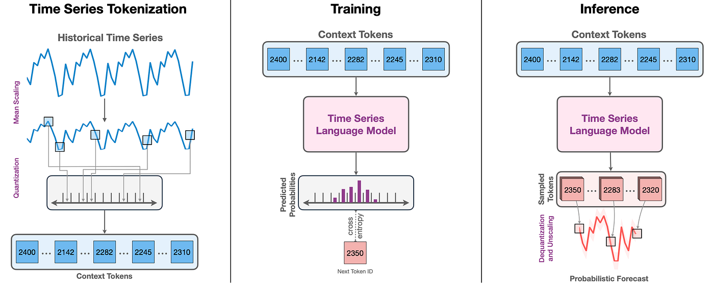
目标时间序列被缩放和量化为一系列令牌。
然后,这些令牌被输入到一个语言模型中,该模型可以是编码器-解码器模型或仅解码器模型。该模型使用交叉熵损失进行训练。
在推理过程中,模型自回归地对令牌进行采样,并将它们映射回数值。通过对多个轨迹进行采样来创建预测分布,从而实现概率预测。
2 ERCOT负荷预测实战
我们首先加载历史ERCOT负荷数据,该数据提供了随时间变化的功耗(负荷)。数据存储在CSV文件中,其中每条记录对应一个时间戳和相应的负荷值。
Chronos无法通过pypi安装。请使用以下命令进行安装:pip install git+https://github.com/amazon-science/chronos-forecasting.git
import matplotlib.pyplot as plt
import numpy as np
import pandas as pd
import torch
from sklearn.model_selection import TimeSeriesSplit
from chronos import ChronosPipeline
df = pd.read_csv("ercot_load_data.csv")
context = torch.tensor(df["values"].values)在这段代码中,我们将数据加载到一个DataFrame中,并重点关注包含负荷数据的values列。然后,我们将这些值转换为PyTorch张量,这是Chronos模型所需的格式。
由于时间序列数据具有时间结构,因此在拆分数据时必须保留这种结构。我们使用sklearn中的TimeSeriesSplit来执行保持时间顺序不变的拆分。
prediction_length = 96
tscv = TimeSeriesSplit(n_splits=2, test_size=prediction_length)
for train_index, test_index in tscv.split(df):
train, test = df.iloc[train_index], df.iloc[test_index]
train_context = torch.tensor(train["values"].values)在这里,我们将prediction_length定义为96,这意味着我们的模型将预测接下来的96个时间步,因为观测值是每15分钟一次(所以每天有96个观测值)。Chronos会警告您,该模型并未针对如此长的预测窗口进行优化。
数据准备好后,我们从Amazon Chronos加载一个预训练的预测模型。该模型基于T5,一种基于transformer的架构,并已准备好在时间序列数据上进行微调。Chronos在有gpu和cuda的情况下表现更好。但我可以在我的笔记本电脑和Google Colab上使用cpu正常运行它。
pipeline = ChronosPipeline.from_pretrained(
"amazon/chronos-t5-small",
device_map="cpu",
torch_dtype=torch.bfloat16,
)
forecast = pipeline.predict(train_context, prediction_length)我们使用ChronosPipeline.from_pretrained()来加载一个为时间序列预测量身定制的预训练T5模型。predict方法根据训练上下文生成接下来prediction_length个步骤的预测。
为了评估模型的性能,我们计算了平均绝对百分比误差(MAPE),这是预测准确性的常用指标。我们将预测值(中位数预测)与测试集中的真实值进行比较。
low, median, high = np.quantile(forecast[0].numpy(), [0.1, 0.5, 0.9], axis=0)
true_values = test["values"].values
mape = np.mean(np.abs((true_values - median) / true_values)) * 100
print(f"MAPE: {mape:.2f}%")
MAPE: 1.27%预测输出是一个预测值数组,我们从中提取第10个百分位数(low)、第50个百分位数(median)和第90个百分位数(high),以表示预测中的不确定性范围。然后,我们计算MAPE,它以百分比的形式告诉我们我们的预测与真实值的接近程度。
最后,我们使用Matplotlib将预测值、历史数据和真实值可视化。
plt.figure(figsize=(10, 5))
plt.plot(df.index, df["values"], color="royalblue", label="历史数据")
plt.plot(test.index, true_values, color="green", label="真实值", linestyle="dashed")
plt.plot(test.index, median, color="red", label="中位数预测")
plt.fill_between(test.index, low, high, color="red", alpha=0.3, label="80%预测区间")
plt.xlabel("时间")
plt.ylabel("负荷")
plt.legend()
plt.title("ERCOT负荷预测")
plt.show()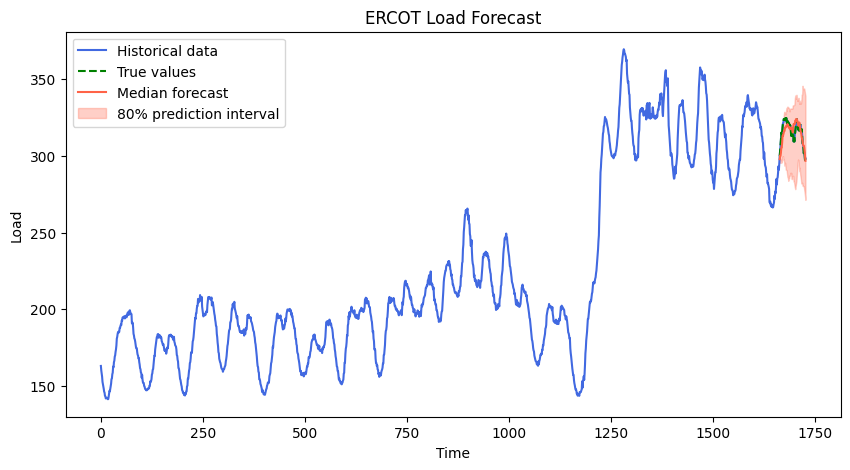
Chronos能够很好地模拟这种负载的波动。
亚马逊Chronos在预测这个真实世界的数据集方面做得非常出色。Chronos与传统时间序列之间的关键区别在于该模型是预先训练好的。我们不是在创建模型。在这个流程中,我们的任务只是推理。这简化了很多事情,但也放弃了很多控制权。
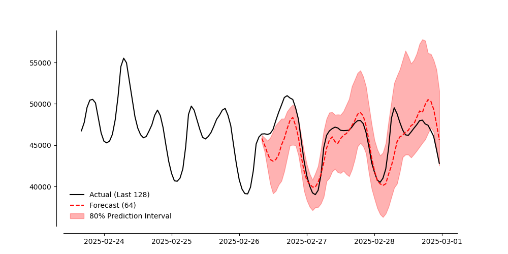
3 更多实验
我使用一个更大的数据集对此进行了更多实验,即2018年至2025年2月的Ercot每小时负荷。结果还不错。
import matplotlib.pyplot as plt
import numpy as np
import pandas as pd
import torch
from chronos import ChronosPipeline
def mape(actual, predicted):
return np.mean(np.abs((actual - predicted) / actual)) * 100
df = pd.read_csv("Ercot_Native_Load_2025 (1).csv")
df["Date"] = pd.to_datetime(df["Date"])
series = df["ERCOT"].values
dates = df["Date"].values
hold_out_length = 64
train_series = series[:-hold_out_length]
actual_holdout = series[-hold_out_length:]
pipeline = ChronosPipeline.from_pretrained(
"amazon/chronos-t5-small",
device_map="cpu",
torch_dtype=torch.bfloat16,
)
context = torch.tensor(train_series, dtype=torch.float32).unsqueeze(0)
forecast = pipeline.predict(context, hold_out_length)
low, median, high = np.quantile(forecast[0].numpy(), [0.1, 0.5, 0.9], axis=0)
plot_range = 64 * 2
plot_series = series[-plot_range:]
plot_dates = dates[-plot_range:]
forecast_dates = dates[-hold_out_length:]
error = mape(actual_holdout, median)
print(f"MAPE: {error:.2f}%")
plt.figure(figsize=(10, 5))
plt.plot(plot_dates, plot_series, color="black", label="实际值(最近128个)")
plt.plot(forecast_dates, median, color="red", linestyle="dashed", label="预测值(64个)")
plt.fill_between(forecast_dates, low, high, color="red", alpha=0.3, label="80%预测区间")
plt.xticks(rotation=45, fontsize=10, fontname="serif")
plt.yticks(fontsize=10, fontname="serif")
plt.gca().spines["top"].set_visible(False)
plt.gca().spines["right"].set_visible(False)
plt.gca().spines["left"].set_position(("outward", 10))
plt.gca().spines["bottom"].set_position(("outward", 10))
plt.legend(frameon=False, fontsize=10)
plt.savefig("ercot_forecast_vs_actual_with_dates.png")
plt.show()
4 美国能源发电数据预测
我用一个不同的数据集重新审视了Chronos。下面是使用有关美国能源发电的数据的代码。
import numpy as np
import pandas as pd
import matplotlib.pyplot as plt
from pathlib import Path
from dataclasses import dataclass
import torch
np.random.seed(42)
plt.rcParams.update({'font.family': 'serif','axes.spines.top': False,'axes.spines.right': False,'axes.linewidth': 0.8})
def save_fig(path: str):
plt.tight_layout(); plt.savefig(path, bbox_inches='tight'); plt.close()
@dataclass
class Config:
csv_path: str = "2001-2025 Net_generation_United_States_all_sectors_monthly.csv"
freq: str = "MS"
horizon: int = 8
model_id: str = "amazon/chronos-t5-tiny"
def load_series(cfg: Config) -> pd.Series:
p = Path(cfg.csv_path)
df = pd.read_csv(p, header=None, usecols=[0,1], names=["date","value"], sep=",")
df["date"] = pd.to_datetime(df["date"], format="%Y-%m-%d", errors="coerce")
df["value"] = pd.to_numeric(df["value"], errors="coerce")
s = df.dropna().sort_values("date").set_index("date")["value"].asfreq(cfg.freq)
return s.astype(float)
def main():
cfg = Config()
y = load_series(cfg)
end_2024 = pd.Timestamp("2024-12-01")
jan_2025 = pd.Timestamp("2025-01-01")
aug_2025 = pd.Timestamp("2025-08-01")
y_train = y.loc[:end_2024]
y_act = y.loc[jan_2025:aug_2025]
try:
from chronos import ChronosPipeline
except Exception:
from chronos_forecasting import ChronosPipeline
pipe = ChronosPipeline.from_pretrained(cfg.model_id, device_map="cpu")
arr = y_train.values.astype(np.float32)
context = torch.tensor(arr, dtype=torch.float32, device="cpu")
out = pipe.predict(context, prediction_length=cfg.horizon)
out_np = np.asarray(out)
if out_np.size % cfg.horizon == 0:
out_np = out_np.reshape(-1, cfg.horizon).mean(axis=0)
else:
out_np = out_np.ravel()[:cfg.horizon]
dates = pd.period_range('2025-01', '2025-08', freq='M').to_timestamp()
fc = pd.Series(out_np, index=dates)
start_2024 = pd.Timestamp("2024-01-01")
y_hist = y.loc[start_2024:end_2024]
fig, ax = plt.subplots(figsize=(10,5))
ax.plot(y_hist.index, y_hist.values, color="#888888", lw=1.5)
ax.axvline(jan_2025, color="#666666", linestyle="--", lw=1)
if len(y_act):
ax.plot(y_act.index, y_act.values, color="#444444", lw=1.8)
ax.plot(fc.index, fc.values, color="#000000", lw=2.0)
from matplotlib.ticker import MaxNLocator, StrMethodFormatter
ax.yaxis.set_major_locator(MaxNLocator(4))
ax.yaxis.set_major_formatter(StrMethodFormatter('{x:,.0f}'))
ax.spines['top'].set_visible(False)
ax.spines['right'].set_visible(False)
ax.grid(False)
ax.set_xlabel('')
if len(y_hist):
ax.annotate('历史 (2024)', xy=(y_hist.index[-1], y_hist.values[-1]), xytext=(6,0), textcoords='offset points', fontsize=9, va='center', ha='left', color='#666666')
if len(y_act):
ax.annotate('实际 (2025年1月–8月)', xy=(y_act.index[-1], y_act.values[-1]), xytext=(6,0), textcoords='offset points', fontsize=9, va='center', ha='left', color='#444444')
ax.annotate('Chronos', xy=(fc.index[-1], fc.values[-1]), xytext=(6,0), textcoords='offset points', fontsize=9, va='center', ha='left', color='#000000')
ax.set_title('EIA净发电量 — Chronos 2025年1月–8月预测')
save_fig('eia_chronos_last_fold.png')
if __name__ == '__main__':
main()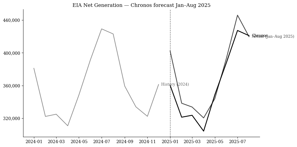

 浙公网安备 33010602011771号