详细介绍：生成模型实战 | 实时任意风格迁移

生成模型实战 | 实时任意风格迁移

• • 0. 前言
  • 1. 自适应实例归一化
  • 2. 风格迁移网络架构
  • 3. 构建编码器
  • 4. 构建解码器
  • 5. 构建风格迁移网络

0. 前言

我们已经学习了如何使用条件实例归一化来传输固定数量的风格。在本节中，我们将实现自适应实例归一化 (adaptive instance normalization, AdaIN)，以使用多样性的风格执行风格迁移。

1. 自适应实例归一化

自适应实例归一化 (adaptive instance normalization, AdaIN) 也是条件实例归一化 (conditional instance normalization, CIN) 的一种，这意味着均值和标准差是在每个图像和每个通道 (H, W) 上计算的，而批归一化是在 (N, H, W) 上计算的。在 CIN 中，$\gamma$ 和 $\beta$ 系数是可训练的变量，它们学习不同风格所需的均值和方差。在 AdaIN 中，$\gamma$ 和 $\beta$ 被风格特征的标准差和均值所取代：
$$AdaIN(x,y)=\sigma (y)\frac{x-\mu (x)}{\sigma (x)}+\mu (y)$$
AdaIN 可以理解为条件实例规范化的一种形式，其中条件是风格特征而不是风格标签。在训练和推理时，我们使用 VGG 提取风格层输出并将其统计信息用作风格条件，这样避免了只能预先定义一组固定风格。使用 PyTorch 实现 AdaIN 函数：

import os
import random
from PIL import Image
from tqdm import tqdm
import torch
import torch.nn as nn
import torch.nn.functional as F
from torch.utils.data import Dataset, DataLoader
import torchvision.transforms as transforms
import torchvision.models as models
import torchvision.utils as vutils
import torchvision
# device
device = torch.device("cuda" if torch.cuda.is_available() else "cpu")
# ImageNet normalization for VGG
imagenet_mean = torch.tensor([0.485, 0.456, 0.406]).view(1,3,1,1).to(device)
imagenet_std  = torch.tensor([0.229, 0.224, 0.225]).view(1,3,1,1).to(device)
def normalize_batch(batch):
return (batch - imagenet_mean) / imagenet_std
def denormalize_batch(batch):
# inverse of normalize, clamp to [0,1]
batch = batch * imagenet_std + imagenet_mean
return torch.clamp(batch, 0, 1)
def calc_mean_std(feat, eps=1e-5):
# feat: N x C x H x W
N, C = feat.size()[:2]
feat_var = feat.view(N, C, -1).var(dim=2, unbiased=False) + eps
std = feat_var.sqrt().view(N, C, 1, 1)
mean = feat.view(N, C, -1).mean(dim=2).view(N, C, 1, 1)
return mean, std
def adaptive_instance_normalization(content_feat, style_feat):
"""AdaIN: align content feature's channelwise mean/std to style's"""
c_mean, c_std = calc_mean_std(content_feat)
s_mean, s_std = calc_mean_std(style_feat)
normalized = (content_feat - c_mean) / c_std
return normalized * s_std + s_mean

可以看出，adaptive_instance_normalization() 是对 AdaIN 方程式的直接实现。其中 calc_mean_std 用于计算特征图的均值和方差，还使用 view() 方法使结果保持四个维度，形状为 (N, 1, 1, C)，而不是默认值 (N, C)。接下来，我们将 AdaIN 整合到风格迁移中。

2. 风格迁移网络架构

下图显示了风格迁移网络的架构和训练管道：

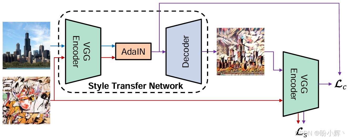
风格迁移网络 (style transfer network, STN) 是编码器/解码器网络，其中，编码器使用固定的 VGG 对内容和风格特征进行编码。然后，AdaIN 将风格特征编码至内容特征的统计信息，然后解码器采用这些新特征来生成风格化图像。

3. 构建编码器

使用 VGG 构建编码器：

class VGGEncoder(nn.Module):
def __init__(self):
super().__init__()
vgg = models.vgg19(weights=torchvision.models.VGG19_Weights.DEFAULT).features
# indices: up to relu4_1 (this slicing is commonly used)
self.enc_layers = nn.Sequential(*[vgg[i] for i in range(21)])
for p in self.enc_layers.parameters():
p.requires_grad = False
def forward(self, x):
return self.enc_layers(x)
def get_vgg_features(x, vgg):
features = []
vgg_full = models.vgg19(weights=torchvision.models.VGG19_Weights.DEFAULT).features.to(device)
vgg_full.eval()
h = x
# we will collect at layer indices corresponding to relu1_1, relu2_1, relu3_1, relu4_1
collect_indices = [1, 6, 11, 20]  # these index choices match common mapping
for i, layer in enumerate(vgg_full):
h = layer(h)
if i in collect_indices:
features.append(h)
if i == 20:
break
return features

4. 构建解码器

尽管我们在编码器代码中使用了 4 个 VGG 层 (block1_conv1 到 block4_conv1)，但 AdaIN 仅使用编码器的最后一层 block4_conv1。因此，解码器的输入张量具有与 block4_conv1 相同的激活。解码器架构由卷积和上采样层组成：

class Decoder(nn.Module):
"""
A decoder that mirrors part of VGG; simple Upsample + Conv blocks.
Input channels: 512 -> output: 3
"""
def __init__(self):
super().__init__()
# we design a reasonable decoder; channel sizes inspired by VGG
self.model = nn.Sequential(
# input: 512 x H x W
nn.Conv2d(512, 256, 3, 1, 1),
nn.ReLU(inplace=True),
nn.Upsample(scale_factor=2, mode='nearest'),  # 256 -> up
nn.Conv2d(256, 256, 3, 1, 1),
nn.ReLU(inplace=True),
nn.Conv2d(256, 256, 3, 1, 1),
nn.ReLU(inplace=True),
nn.Conv2d(256, 256, 3, 1, 1),
nn.ReLU(inplace=True),
nn.Conv2d(256, 128, 3, 1, 1),
nn.ReLU(inplace=True),
nn.Upsample(scale_factor=2, mode='nearest'),  # up
nn.Conv2d(128, 128, 3, 1, 1),
nn.ReLU(inplace=True),
nn.Conv2d(128, 64, 3, 1, 1),
nn.ReLU(inplace=True),
nn.Upsample(scale_factor=2, mode='nearest'),  # up
nn.Conv2d(64, 64, 3, 1, 1),
nn.ReLU(inplace=True),
nn.Conv2d(64, 3, 3, 1, 1),
# output no activation; we'll clamp later
)
def forward(self, x):
return self.model(x)

除不具有任何非线性激活功能的输出层外，所有层均使用 ReLU 激活功能。现在，我们已经完成了 AdaIN，编码器和解码器，并且可以继续进行图像预处理流程了。现在，我们已经准备好所有构件，剩下要做的就是将它们放在一起以创建 STN 和训练管道。

5. 构建风格迁移网络

(1) 定义数据集加载器：

class ImageFolderDataset(Dataset):
def __init__(self, folder, transform):
super().__init__()
self.files = []
for root, _, fnames in os.walk(folder):
for f in fnames:
if f.lower().endswith(('png', 'jpg', 'jpeg', 'bmp')):
self.files.append(os.path.join(root, f))
self.transform = transform
def __len__(self):
return len(self.files)
def __getitem__(self, idx):
path = self.files[idx]
img = Image.open(path).convert('RGB')
return self.transform(img)
class ContentStyleDataset(Dataset):
"""
Returns a pair (content, style) by sampling from content_dir and style_dir.
"""
def __init__(self, content_dir, style_dir, size=256):
self.content_ds = ImageFolderDataset(content_dir, transforms.Compose([
transforms.Resize(int(size*1.15)),
transforms.RandomCrop(size),
transforms.ToTensor()
]))
self.style_ds = ImageFolderDataset(style_dir, transforms.Compose([
transforms.Resize(int(size*1.15)),
transforms.RandomCrop(size),
transforms.ToTensor()
]))
def __len__(self):
return max(len(self.content_ds), len(self.style_ds))
def __getitem__(self, idx):
c = self.content_ds[idx % len(self.content_ds)]
s = self.style_ds[random.randint(0, len(self.style_ds)-1)]
return c, s

(2) 构造 STN 非常简单，只需连接编码器，AdaIN 和解码器即可，如以上架构图所示。 STN 还是我们将用来执行推理的模型：

def train_adain(content_dir, style_dir, save_dir,
image_size=256, batch_size=8, epochs=10,
content_weight=1.0, style_weight=10.0, lr=1e-4,
save_every=1000):
os.makedirs(save_dir, exist_ok=True)
# datasets & loaders
dataset = ContentStyleDataset(content_dir, style_dir, size=image_size)
dataloader = DataLoader(dataset, batch_size=batch_size, shuffle=True, num_workers=4, drop_last=True)
# models
vgg = VGGEncoder().to(device).eval()
# freeze a separate full-vgg for multi-layer features
vgg_full = models.vgg19(weights=torchvision.models.VGG19_Weights.DEFAULT).features.to(device).eval()
for p in vgg_full.parameters():
p.requires_grad = False
decoder = Decoder().to(device)
optimizer = torch.optim.Adam(decoder.parameters(), lr=lr)
iter_count = 0
for epoch in range(epochs):
pbar = tqdm(dataloader, desc=f"Epoch {epoch+1}/{epochs}")
for content, style in pbar:
iter_count += 1
content = content.to(device)
style = style.to(device)
# normalize for vgg
c_in = normalize_batch(content)
s_in = normalize_batch(style)
# extract features
with torch.no_grad():
c_feat = vgg.forward(c_in)
s_feat = vgg.forward(s_in)
# compute AdaIN target (t)
t = adaptive_instance_normalization(c_feat, s_feat)
t = t.detach()  # do not backprop through encoder
# decode
g = decoder(t)
# content loss: compare features of generated g and t at relu4_1
g_in = normalize_batch(g)
def extract_multifeats(x):
feats = []
h = x
collect_indices = [1, 6, 11, 20]
for i, layer in enumerate(vgg_full):
h = layer(h)
if i in collect_indices:
feats.append(h)
if i == 20:
break
return feats
with torch.no_grad():
# style feats from original style image
s_feats = extract_multifeats(s_in)
g_feats = extract_multifeats(g_in)
content_loss = F.mse_loss(g_feats[-1], t)
# style loss: compare mean/std of g_feats and s_feats
style_loss = style_loss_from_features(g_feats, s_feats)
loss = content_weight * content_loss + style_weight * style_loss
optimizer.zero_grad()
loss.backward()
optimizer.step()
pbar.set_postfix({
'loss': f"{loss.item():.4f}",
'c_loss': f"{content_loss.item():.4f}",
's_loss': f"{style_loss.item():.4f}"
})
if iter_count % save_every == 0:
torch.save(decoder.state_dict(), os.path.join(save_dir, f"decoder_iter_{iter_count}.pth"))
print(f"Saved decoder at iter {iter_count}")
# final save
torch.save(decoder.state_dict(), os.path.join(save_dir, "decoder_final.pth"))
print("Training finished, model saved.")

内容和风格图像经过预处理，然后送入编码器。最后一个特征层 block4_conv1 进入 AdaIN()。然后风格化特征进入解码器以生成 RGB 风格化的图像。

(3) 内容损失和风格损失是根据固定 VGG 提取的激活来计算的。内容损失是 L2 范数，将生成的风格化图像的内容特征与 AdaIN 的输出进行比较，这使收敛速度更快。对于风格损失，将常用的 Gram 矩阵替换为均值和方差激活统计的 L2 范数。这产生的结果类似于 Gram 矩阵，但从概念上讲更清晰。以下是风格损失函数方程：
$${\mathcal{L}}_s=\sum _{i=1}^L||\mu ({\varphi }_i(stylized))-\mu ({\varphi }_i(style))|{|}_2+||\sigma ({\varphi }_i(stylized))-\sigma ({\varphi }_i(style))|{|}_2$$
其中，${\varphi }_i$ 表示 VGG-19 中用于计算风格损失的层。
我们使用 calc_mean_std() 来计算来自风格化图像和风格图像的特征之间的统计量和 L2 范数，对内容层的损失求均值：

def style_loss_from_features(generated_feats, style_feats):
# both lists for multiple layers
loss = 0.0
for gf, sf in zip(generated_feats, style_feats):
gm, gs = calc_mean_std(gf)
sm, ss = calc_mean_std(sf)
loss += F.mse_loss(gm, sm) + F.mse_loss(gs, ss)
return loss

(4) 实现模型推理管道：

from torchvision.transforms.functional import to_pil_image
def load_image(path, size=512):
img = Image.open(path).convert('RGB')
transform = transforms.Compose([
transforms.Resize(size),
transforms.CenterCrop(size),
transforms.ToTensor()
])
return transform(img).unsqueeze(0).to(device)  # 1 x 3 x H x W
def stylize(content_path, style_path, decoder, vgg, alpha=1.0, size=512):
c = load_image(content_path, size=size)
s = load_image(style_path, size=size)
c_in = normalize_batch(c)
s_in = normalize_batch(s)
with torch.no_grad():
c_feat = vgg(c_in)
s_feat = vgg(s_in)
t = adaptive_instance_normalization(c_feat, s_feat)
t = alpha * t + (1 - alpha) * c_feat
g = decoder(t)
img = denormalize_batch(g).cpu().squeeze(0)
pil = to_pil_image(img)
return pil

(5) 最后，实现主函数：

if __name__ == '__main__':
import argparse
parser = argparse.ArgumentParser()
parser.add_argument('--content_dir', type=str, default='data/content')
parser.add_argument('--style_dir', type=str, default='data/style')
parser.add_argument('--save_dir', type=str, default='checkpoints')
parser.add_argument('--mode', type=str, default='train', choices=['train', 'stylize'])
parser.add_argument('--content_image', type=str, default='')
parser.add_argument('--style_image', type=str, default='')
parser.add_argument('--alpha', type=float, default=1.0)
parser.add_argument('--image_size', type=int, default=256)
args = parser.parse_args()
if args.mode == 'train':
train_adain(args.content_dir, args.style_dir, args.save_dir,
image_size=args.image_size, batch_size=8, epochs=10,
content_weight=1.0, style_weight=10.0, lr=1e-4, save_every=2000)
else:
# load decoder
decoder = Decoder().to(device)
# load checkpoint - make sure path exists
ckpt = os.path.join(args.save_dir, 'decoder_final.pth')
if not os.path.exists(ckpt):
raise RuntimeError("Please train model or provide checkpoint path")
decoder.load_state_dict(torch.load(ckpt, map_location=device))
vgg = VGGEncoder().to(device).eval()
out = stylize(args.content_image, args.style_image, decoder, vgg, alpha=args.alpha, size=512)
out.save('stylized_result.png')
print("Stylized image saved to stylized_result.png")

我们将内容权重固定为 1，并调整风格权重，在此示例中，我们将风格权重设置为 1e-4。在网络架构中，看起来好像有三个要训练的网络，但是其中两个是固定的 VGG，因此唯一可训练的网络是解码器。因此，我们仅跟踪梯度并将其应用于解码器。

(6) 在本节中，将使用 CelebA 人脸图像 作为内容图像，并使用 Best Artworks of All Time 作为风格图像。Best Artworks of All Time 数据集收录了 50 位历史上极具影响力的艺术家的作品，包含约 12000 张画作图像。数据集下载完成后，将内容图像和风格图像分别放在 data/content 和 data/style 目录下，使用以下命令启动训练过程：

$ python3 adain_train.py --content_dir data/content --style_dir data/style

训练完成后，使用以下命令生成风格化图像：

python3 adain_train.py --mode stylize --content_image data/content/016280.jpg --style_image data/style/test/Vincent_van_Gogh_875.jpg --alpha 10.0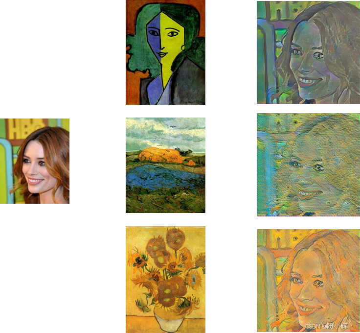

上图中的图像显示了使用网络训练时未看到的风格图像在推理时进行风格迁移的情况。每种风格转移仅通过单个前向计算进行，这比原始神经风格迁移算法的迭代优化快得多。