数据挖掘2

1、

import numpy as np
import pandas as pd

inputfile = 'D:/WeixinWenjian/WeChat Files/wxid_5onnacvxxvpj22/FileStorage/File/2023-03/data.csv'
data = pd.read_csv(inputfile)

description = [data.min(),data.max(),data.mean(),data.std()]

description = pd.DataFrame(description,index = ['Min','Max','Mean','STD']).T
print('描述性统计结果：\n',np.round(description,2))

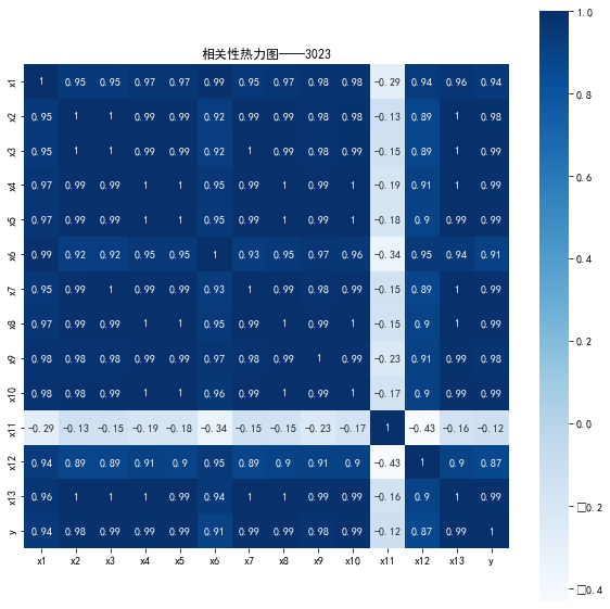
corr = data.corr(method='pearson')
print('相关系数矩阵为：\n',np.round(corr,2))

import matplotlib.pyplot as plt
import seaborn as sns
plt.subplots(figsize=(10,10))
sns.heatmap(corr,annot=True,vmax=1,square=True,cmap="Blues")
plt.rcParams['font.sans-serif'] = 'SimHei'
plt.title('相关性热力图——3023')
plt.show()
plt.close

 

 

2、

import numpy as np
import pandas as pd
from sklearn.linear_model import Lasso

inputfile = 'D:/WeixinWenjian/WeChat Files/wxid_5onnacvxxvpj22/FileStorage/File/2023-03/data.csv'
data = pd.read_csv(inputfile)
lasso = Lasso(1000)
lasso.fit(data.iloc[:,0:13],data['y'])
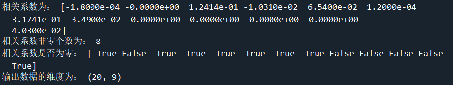
print('相关系数为：',np.round(lasso.coef_,5))

print('相关系数非零个数为：',np.sum(lasso.coef_ !=0))
mask = lasso.coef_ != 0
print('相关系数是否为零：',mask)
mask = np.append(mask, True)

outputfile = 'D:/WeixinWenjian/WeChat Files/wxid_5onnacvxxvpj22/FileStorage/File/2023-03/data2.csv'
new_reg_data = data.iloc[:,mask]
new_reg_data.to_csv(outputfile)
print('输出数据的维度为：',new_reg_data.shape)

 

 

3、

import sys
sys.path.append('D:/WeixinWenjian/WeChat Files/wxid_5onnacvxxvpj22/FileStorage/File/2023-03')
import numpy as np
import pandas as pd
from GM11 import GM11

inputfile1 = 'D:/WeixinWenjian/WeChat Files/wxid_5onnacvxxvpj22/FileStorage/File/2023-03/data2.csv'
inputfile2 = 'D:/WeixinWenjian/WeChat Files/wxid_5onnacvxxvpj22/FileStorage/File/2023-03/data.csv'
new_reg_data = pd.read_csv(inputfile1)
data = pd.read_csv(inputfile2)
new_reg_data.index = range(1994, 2014)
new_reg_data.loc[2014] = None
new_reg_data.loc[2015] = None
new_reg_data.loc[2016] = None

l = ['x1', 'x3', 'x4', 'x5', 'x6', 'x7', 'x8', 'x13']
for i in l:
f = GM11(new_reg_data.loc[range(1994, 2014),i].to_numpy())[0]
new_reg_data.loc[2014,i] = f(len(new_reg_data)-2)
new_reg_data.loc[2015,i] = f(len(new_reg_data)-1)
new_reg_data.loc[2016,i] = f(len(new_reg_data))
new_reg_data[i] = new_reg_data[i].round(2)

outputfile = 'D:/WeixinWenjian/WeChat Files/wxid_5onnacvxxvpj22/FileStorage/File/2023-03/data_GM21.xls'
y = list(data['y'].values)
y.extend([np.nan,np.nan,np.nan])
new_reg_data['y'] = y

new_reg_data.to_excel(outputfile)
print('预测结果为：\n',new_reg_data.loc[2014:2016,:])

import matplotlib.pyplot as plt
from sklearn.svm import LinearSVR

inputfile = 'D:/WeixinWenjian/WeChat Files/wxid_5onnacvxxvpj22/FileStorage/File/2023-03/data_GM21.xls' 
data = pd.read_excel(inputfile) 
feature = ['x1', 'x3', 'x4', 'x5', 'x6', 'x7', 'x8', 'x13'] 
data_train = data.iloc[0:20,:].copy() 

data_mean = data_train.mean()
data_std = data_train.std()

data_train = (data_train - data_mean)/data_std 
x_train = data_train[feature].to_numpy() 
y_train = data_train['y'].to_numpy() 

linearsvr = LinearSVR() 
linearsvr.fit(x_train,y_train)

x = ((data[feature] - data_mean[feature])/data_std[feature]).to_numpy() 
data['y_pred'] = linearsvr.predict(x) * data_std['y'] + data_mean['y']
outputfile = 'D:/WeixinWenjian/WeChat Files/wxid_5onnacvxxvpj22/FileStorage/File/2023-03/data_GM21_revenue.xls' 
data.to_excel(outputfile)
plt.rcParams['font.sans-serif'] = ['SimHei'];
print('真实值与预测值分别为：\n',data[['y','y_pred']])

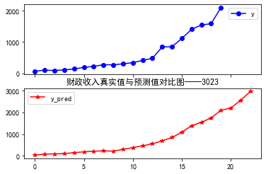
fig = data[['y','y_pred']].plot(subplots = True, style=['b-o','r-*']) 
plt.title('财政收入真实值与预测值对比图——3023')
plt.show()