航空公司客户价值分析

import pandas as pd
datafile = 'E:\py mathph\JupyterLab-Portable-3.1.0-3.9\shujuwajue/air_data.csv'#航空公司原始数据，第一行是属性名
resultfile = 'E:\py mathph\JupyterLab-Portable-3.1.0-3.9\shujuwajue/explore.xlsx'
data = pd.read_csv(datafile, encoding='utf-8')
explore = data.describe( percentiles = [],include = 'all').T
explore['null'] = len(data)-explore['count']
explore1 = explore[['null','max','min']]
explore1.columns = [u'空值数',u'最大值',u'最小值']#重命名列名
explore1.to_excel(resultfile)

　　

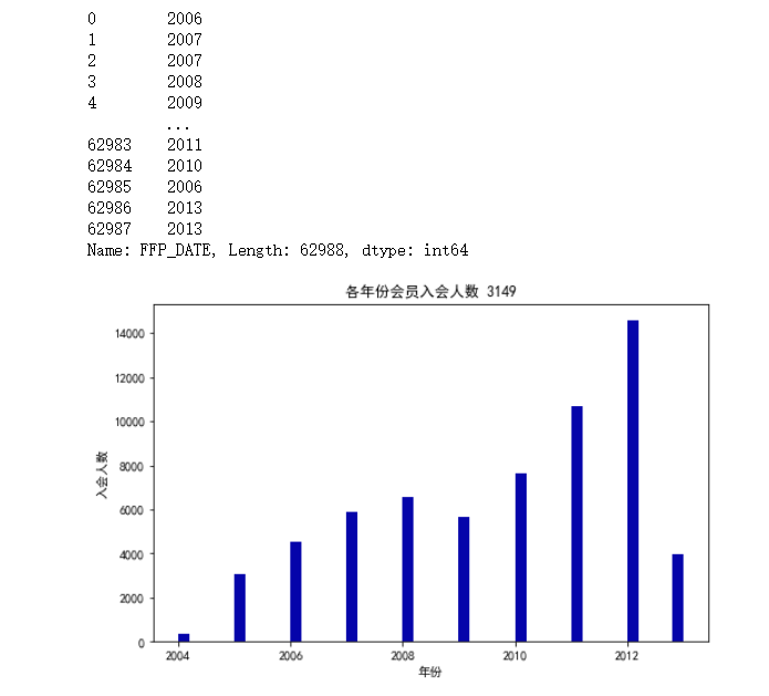
import matplotlib.pyplot as plt
from datetime import datetime 
#客户信息类别
#提取会员入会年份
ffp = data['FFP_DATE'].apply(lambda x:datetime.strptime(x, '%Y/%m/%d'))
ffp_year = ffp.map(lambda x : x.year)
print(ffp_year)
#绘制各年份会员入会人数直方图
fig = plt.figure(figsize=(8, 5))  #设置画布大小
plt.rcParams['font.sans-serif'] = ['SimHei']  #用来正常显示中文标签
plt.rcParams['axes.unicode_minus'] = False  #用来正常显示负号#探索客户的基本信息分布情况
plt.hist(ffp_year, bins='auto', color='#0504aa')
plt.xlabel('年份')
plt.ylabel('入会人数')
plt.title('各年份会员入会人数 3149')
plt.show()
plt.close()

 

 

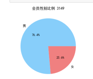
#提取会员不同性别人数
male = pd.value_counts(data['GENDER'])['男']
female = pd.value_counts(data['GENDER'])['女']
#绘制会员性别比例饼图
fig = plt.figure(figsize=(7, 4))  #设置画布大小
plt.pie([male, female], labels=['男', '女'], colors=['lightskyblue', 'lightcoral'], autopct='%1.1f%%')
plt.title('会员性别比例 3149')
plt.show()
plt.close()

 

 

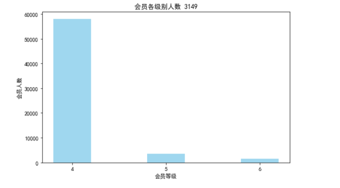
#提取不同级别会员的人数
lv_four = pd.value_counts(data['FFP_TIER'])[4]
lv_five = pd.value_counts(data['FFP_TIER'])[5]
lv_six = pd.value_counts(data['FFP_TIER'])[6]
#绘制会员各级别人数条形图
fig = plt.figure(figsize=(8,5))  #设置画布大小
plt.bar(range(3), [lv_four, lv_five, lv_six], width=0.4, alpha=0.8, color='skyblue')
#left：x轴的位置序列，一般采用arange函数产生一个序列；
#height：y轴的数值序列，也就是柱形图的高度，一般就是我们需要展示的数据；
#alpha：透明度
#width：为柱形图的宽度，一般这是为0.8即可；
#color或facecolor：柱形图填充的颜色；
plt.xticks([index for index in range(3)], ['4', '5', '6'])
plt.xlabel('会员等级')
plt.ylabel('会员人数')
plt.title('会员各级别人数 3149')
plt.show()
plt.close()

 

 

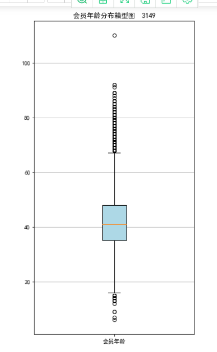
#提取会员年龄
age = data['AGE'].dropna()
age = age.astype('int64')
#绘制会员年龄分布箱型图
fig = plt.figure(figsize=(5,10))
plt.boxplot(age, patch_artist=True, labels=['会员年龄'], boxprops={'facecolor': 'lightblue'}) #设置填充颜色
plt.title('会员年龄分布箱型图  3149')
#显示y坐标轴的底线
plt.grid(axis='y')
plt.show()
plt.close()

 

 

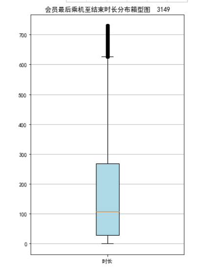
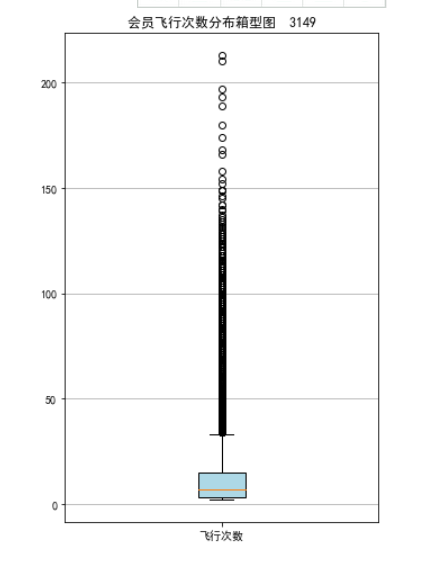
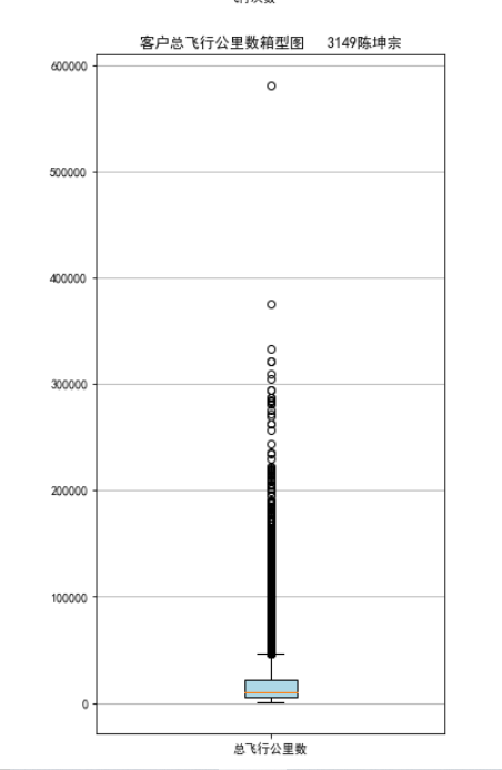
#7-3
lte=data['LAST_TO_END']
fc=data['FLIGHT_COUNT']
sks=data['SEG_KM_SUM']

fig=plt.figure(figsize=(5,8))

plt.boxplot(lte,
            patch_artist=True,
            labels=['时长'],
            boxprops={'facecolor':'lightblue'})
plt.title('会员最后乘机至结束时长分布箱型图  3149')
plt.grid(axis='y')
plt.show()
plt.close

fig=plt.figure(figsize=(5,8))
plt.boxplot(fc,
            patch_artist=True,
            labels=['飞行次数'],
            boxprops={'facecolor':'lightblue'})
plt.title('会员飞行次数分布箱型图  3149')
plt.grid(axis='y')
plt.show()
plt.close

fig=plt.figure(figsize=(5,10))
plt.boxplot(sks,
            patch_artist=True,
            labels=['总飞行公里数'],
            boxprops={'facecolor':'lightblue'})
plt.title('客户总飞行公里数箱型图   3149陈坤宗')
plt.grid(axis='y')
plt.show()
plt.close

 

 

 

 

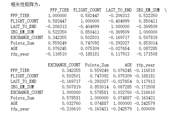
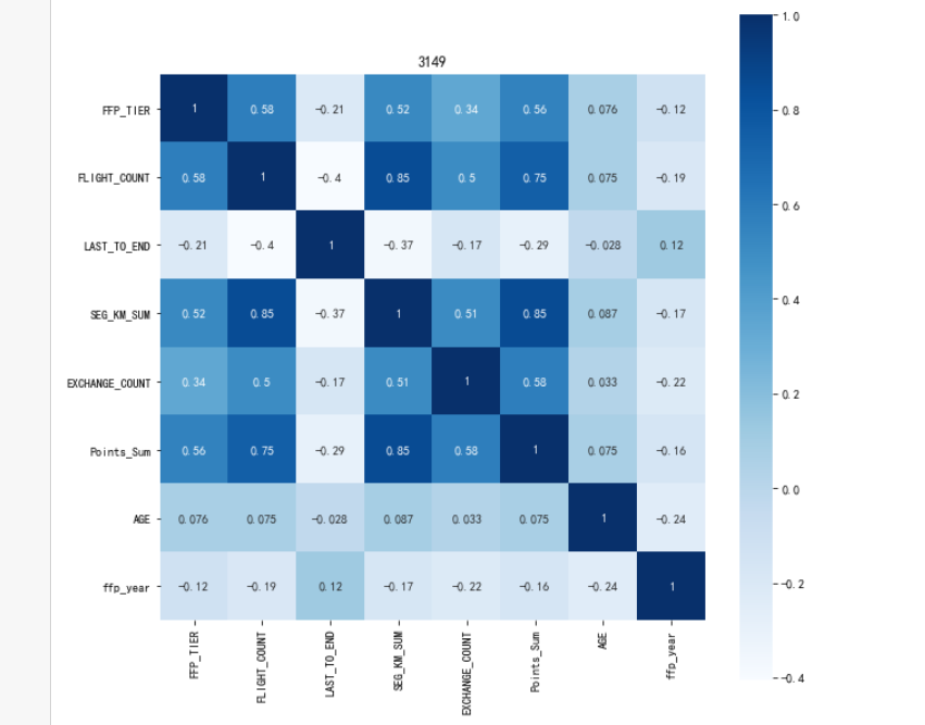
#3相关性分析
#提取属性并合并为新的数据集
data_corr = data.loc[:,['FFP_TIER', 'FLIGHT_COUNT', 'LAST_TO_END', 'SEG_KM_SUM', 'EXCHANGE_COUNT', 'Points_Sum']]
age1 = data['AGE'].fillna(0)
data_corr['AGE'] = age1.astype('int64')
data_corr['ffp_year'] = ffp_year

#计算相关性矩阵
dt_corr = data_corr.corr(method='pearson')
print('相关性矩阵为：\n', dt_corr)

#绘制热力图
import seaborn as sns
plt.subplots(figsize=(10, 10))  #设置画面大小
## data:数据 square:是否是正方形 vmax:最大值 vmin:最小值 robust:排除极端值影响
sns.heatmap(dt_corr, annot=True, vmax=1, square=True, cmap='Blues')
plt.title('3149')
plt.show()
plt.close()

 

 

 

 

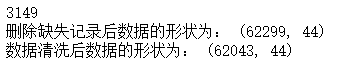
datafile = 'E:\py mathph\JupyterLab-Portable-3.1.0-3.9\shujuwajue/air_data.csv'#航空公司原始数据，第一行是属性名
# 去除票价为空的记录
cleanedfile = 'E:\py mathph\JupyterLab-Portable-3.1.0-3.9\shujuwajue/cleaned.csv'
airline_data = pd.read_csv(datafile, encoding='utf-8')
airline_notnull = airline_data.loc[airline_data['SUM_YR_1'].notnull() & 
                                   airline_data['SUM_YR_2'].notnull(),:]
print('3149 \n删除缺失记录后数据的形状为：',airline_notnull.shape)
# 只保留票价非零的，或者平均折扣率不为0且总飞行公里数大于0的记录。
index1 = airline_notnull['SUM_YR_1'] != 0
index2 = airline_notnull['SUM_YR_2'] != 0
index3 = (airline_notnull['SEG_KM_SUM']> 0) & (airline_notnull['avg_discount'] != 0)
index4 = airline_notnull['AGE'] > 100  # 去除年龄大于100的记录
airline = airline_notnull[(index1 | index2) & index3 & ~index4]
print('数据清洗后数据的形状为：',airline.shape)
airline.to_csv(cleanedfile)  # 保存清洗后的数据

 

 

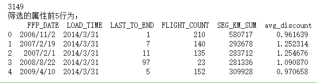
import pandas as pd
import numpy as np

# 读取数据清洗后的数据
cleanedfile = 'E:\py mathph\JupyterLab-Portable-3.1.0-3.9\shujuwajue/cleaned.csv' # 数据清洗后保存的文件路径
airline = pd.read_csv(cleanedfile, encoding='utf-8')
# 选取需求属性
airline_selection = airline[['FFP_DATE', 'LOAD_TIME', 'LAST_TO_END', 'FLIGHT_COUNT', 'SEG_KM_SUM', 'avg_discount']]
print('3149 \n筛选的属性前5行为：\n', airline_selection.head())

 

 

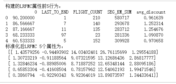
# 7-8 属性构造与数据标准化
# 构造属性L
L = pd.to_datetime(airline_selection['LOAD_TIME']) -  pd.to_datetime(airline_selection['FFP_DATE'])
L = L.astype('str').str.split().str[0]
L = L.astype('int')/30

# 合并属性
airline_features = pd.concat([L,airline_selection.iloc[:,2:]],axis=1)
print('构建的LRFMC属性前5行为：\n', airline_features.head())

# 数据标准化
from sklearn.preprocessing import StandardScaler
data = StandardScaler().fit_transform(airline_features)
np.savez('E:\py mathph\JupyterLab-Portable-3.1.0-3.9\shujuwajue/airline_scale.npz', data)
print('标准化后LRFMC 5个属性为：\n', data[:5,:])

 

 

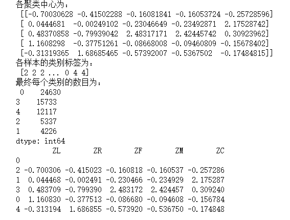
#代码7-9 K-Meas聚类标准化后的数据
import pandas as pd
import numpy as np
from sklearn.cluster import KMeans #导入K-Mmeans算法

#读取标准化后的数据
airline_scale = np.load('E:\py mathph\JupyterLab-Portable-3.1.0-3.9\shujuwajue/airline_scale.npz')['arr_0']
k = 5 #确定聚类中心数

#构建模型，随机种子设为123
kmeans_model = KMeans(n_clusters=k,n_jobs=4,random_state=123)
fit_kmeans = kmeans_model.fit(airline_scale) #模型训练

#查看聚类结果
kmeans_cc = kmeans_model.cluster_centers_ #聚类中心
print('各聚类中心为：\n',kmeans_cc)
kmeans_labels = kmeans_model.labels_ #样本的类别标签
print('各样本的类别标签为：\n',kmeans_labels)
r1 = pd.Series(kmeans_model.labels_).value_counts() #统计不同类别样本的数目
print('最终每个类别的数目为：\n',r1)
#输出聚类分群的结果
cluster_center = pd.DataFrame(kmeans_model.cluster_centers_,\
                             columns = ['ZL','ZR','ZF','ZM','ZC']) #将聚类中心放在数据中
cluster_center.index = pd.DataFrame(kmeans_model.labels_).\
                             drop_duplicates().iloc[:,0] #将样本类别作为数据框索引
print(cluster_center)

 

 

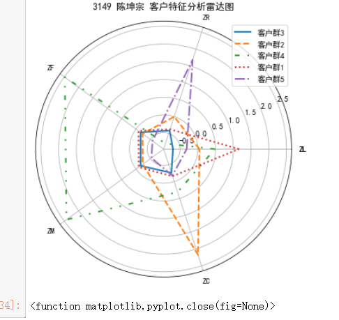
%matplotlib inline
import matplotlib.pyplot as plt
# 客户分群雷达图
labels = ['ZL','ZR','ZF','ZM','ZC']
legen = ['客户群' + str(i + 1) for i in cluster_center.index] # 客户群命名，作为雷达图的图例
lstype = ['-','--',(0, (3, 5, 1, 5, 1, 5)),':','-.']
kinds = list(cluster_center.iloc[:, 0])
# 由于雷达图要保证数据闭合，因此再添加L列，并转换为 np.ndarray
cluster_center = pd.concat([cluster_center, cluster_center[['ZL']]], axis=1)
centers = np.array(cluster_center.iloc[:, 0:])

# 分割圆周长，并让其闭合
n = len(labels)
angle = np.linspace(0, 2 * np.pi, n, endpoint=False)
angle = np.concatenate((angle, [angle[0]]))
labels = np.concatenate((labels, [labels[0]]))
# 绘图
fig = plt.figure(figsize = (8,6))
ax = fig.add_subplot(111, polar=True) # 以极坐标的形式绘制图形
plt.rcParams['font.sans-serif'] = ['SimHei'] # 用来正常显示中文标签
plt.rcParams['axes.unicode_minus'] = False # 用来正常显示负号
# 画线
for i in range(len(kinds)):
    ax.plot(angle, centers[i], linestyle=lstype[i], linewidth=2, label=kinds[i])
# 添加属性标签
ax.set_thetagrids(angle * 180 / np.pi, labels)
plt.title('3149 陈坤宗 客户特征分析雷达图')
plt.legend(legen)
plt.show()
plt.close