
实验一 感知器及其应用
作业信息
| 博客班级 | https://edu.cnblogs.com/campus/ahgc/machinelearning |
|---|---|
| 作业要求 | https://edu.cnblogs.com/campus/ahgc/machinelearning/homework/11950 |
| 作业目标 | 理解并实现感知器算法 |
| 学号 | <3180701337> |
一、实验目的
-
理解感知器算法原理,能实现感知器算法;
-
掌握机器学习算法的度量指标;
-
掌握最小二乘法进行参数估计基本原理;
-
针对特定应用场景及数据,能构建感知器模型并进行预测。
二、实验内容
-
安装Pycharm,注册学生版。
-
安装常见的机器学习库,如Scipy、Numpy、Pandas、Matplotlib,sklearn等。
-
编程实现感知器算法。
-
熟悉iris数据集,并能使用感知器算法对该数据集构建模型并应用。
三、实验报告要求
-
按实验内容撰写实验过程;
-
报告中涉及到的代码,每一行需要有详细的注释;
-
按自己的理解重新组织,禁止粘贴复制实验内容!
四、实验内容
1.代码注释
(1)
import pandas as pd #给引入的包pandas定义一个别名pd
import numpy as np #给引入的包numpy定义一个别名np,上两步是Dataframe创建二维数组
from sklearn.datasets import load_iris #从sklearn包中的datasets类中引入load_iris方法
import matplotlib.pyplot as plt #给包matplotlib.pyplot定义一个plt别名
%matplotlib inline #使用%matplotlib命令可以将matplotlib的图表直接嵌入到Notebook之中,inline表示将图表嵌入到Notebook中。
(2)
# load data
iris = load_iris() #加载数据集(这里使用的是鸢尾花数据集)
df = pd.DataFrame(iris.data, columns=iris.feature_names)  #设置纵列名称为特征
df['label'] = iris.target #增加一列为目标标签
(3)
#
df.columns = ['sepal length', 'sepal width', 'petal length', 'petal width', 'label'] #重命名各个列的名称
df.label.value_counts() #返回数据中其中每个标签取值的个数
(4)
plt.scatter(df[:50]['sepal length'], df[:50]['sepal width'], label='0')  #将数据的前50个数据绘制散点图,令其标签为0
plt.scatter(df[50:100]['sepal length'], df[50:100]['sepal width'], label='1') #将数据的50到100个数据绘制散点图,令其标签为1,这里只选取了0,1两个特征
plt.xlabel('sepal length') #将散点图的x轴命名为sepal length
plt.ylabel('sepal width') #将散点图的y轴命名为sepal width
plt.legend() #显示图例的位置,自适应方式
(5)
data = np.array(df.iloc[:100, [0, 1, -1]]) #选取前100行,第1,2,3列数据,创建数组
(6)
X, y = data[:,:-1], data[:,-1] #X取数据从后向前(相反)的元素,y取date中除了最后一个元素的全部元素
(7)
y = np.array([1 if i == 1 else -1 for i in y]) #将两个类别分别重新设定为+1和-1
(8)
# 数据线性可分,二分类数据
# 此处为一元一次线性方程
class Model: #定义一个类名为Model的类
    def __init__(self): #类Model中有3个变量参数w,b,l_rate
        self.w = np.ones(len(data[0])-1, dtype=np.float32) #将参数w1和w2置为1
        self.b = 0 #将参数b置为0
        self.l_rate = 0.1 #将参数l_rate即学习率置为0.1
        # self.data = data

    def sign(self, x, w, b): #定义sign函数
        y = np.dot(x, w) + b #进行矩阵乘法运算
        return y

    # 随机梯度下降法
    def fit(self, X_train, y_train): #定义fit函数
        is_wrong = False #将误分类点初始化为False
        while not is_wrong: #当is_wrong不符合条件时进行循环
            wrong_count = 0 #误分类点个数初始为0
            for d in range(len(X_train)): #依据X_train行数进行循环
                X = X_train[d]  #取X_train一组及一行数据
                y = y_train[d]  #取y_train一组及一行数据
                if y * self.sign(X, self.w, self.b) <= 0: #判断是否分类错误,若错误,执行下列操作
                    self.w = self.w + self.l_rate*np.dot(y, X) #更新w
                    self.b = self.b + self.l_rate*y #更新b
                    wrong_count += 1 #误分点个数加1
            if wrong_count == 0: #若误分点个数为0
                is_wrong = True #将is_wrong设为True,即跳出循环
        return 'Perceptron Model!'

    def score(self):
        pass
(9)
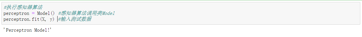
#执行感知器算法
perceptron = Model() #感知器算法调用类Model
perceptron.fit(X, y) #输入测试数据
(10)
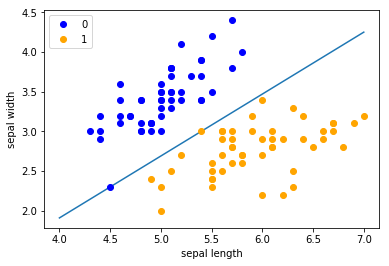
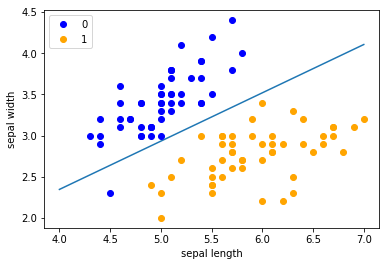
x_points = np.linspace(4, 7,10) #在4到7的闭区间,划分为10个数据点
y_ = -(perceptron.w[0]*x_points + perceptron.b)/perceptron.w[1] #绘制超平面
plt.plot(x_points, y_)

plt.plot(data[:50, 0], data[:50, 1], 'bo', color='blue', label='0') #将前50个数据绘制成散点图
plt.plot(data[50:100, 0], data[50:100, 1], 'bo', color='orange', label='1') # 将50到100之间的数据绘制成散点图
plt.xlabel('sepal length') #散点图横坐标为sepal length
plt.ylabel('sepal width') #散点图纵坐标为sepal length
plt.legend()
(11)
from sklearn.linear_model import Perceptron #将sklearn.linear_model导入到当前的作用域Perceptron即感知器模型中。
(12)
clf = Perceptron(fit_intercept=False, max_iter=1000, shuffle=False)
clf.fit(X, y)
(13)
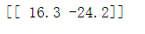
# Weights assigned to the features.
print(clf.coef_) #clf.coef_表示特征的权值的矩阵形式。
(14)
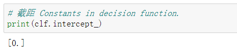
# 截距 Constants in decision function.
print(clf.intercept_)
(15)
x_ponits = np.arange(4, 8) #默认步长为1 输出[4 5 6 7 8]
y_ = -(clf.coef_[0][0]*x_ponits + clf.intercept_)/clf.coef_[0][1] #绘制超平面
plt.plot(x_ponits, y_)
plt.plot(data[:50, 0], data[:50, 1], 'bo', color='blue', label='0') #将前50个数据绘制成散点图
plt.plot(data[50:100, 0], data[50:100, 1], 'bo', color='orange', label='1') # 将50到100之间的数据绘制成散点图
plt.xlabel('sepal length') #散点图横坐标为sepal length
plt.ylabel('sepal width') #散点图纵坐标为sepal length
plt.legend()
2.运行结果
步骤(3)

步骤(4)

步骤(9)
步骤(10)
步骤(12)

步骤(13)
步骤(14)
步骤(15)
五、实验小结
通过本次实验,我对感知器算法的思想与实现方法有了一定的认识。首先感知机是线性分类的二分类模型,输入为实例的特征向量,输出为实例的类别,分
别用 1 和 -1 表示。感知机将输入空间(特征空间)中的实例划分为正负两类分离的超平面,旨在求出将训练集进行线性划分的超平面,为此,导入基于误分
类的损失函数,利用梯度下降法对损失函数进行极小化,求得最优解。这种算法的基本思想是:对于初始的或者迭代中的增广权矢量W,用训练模式检验其合
理性。当不合理时,再利用梯度下降法对其进行校正。

 浙公网安备 33010602011771号