Paper Reading ---- VESPA: Static Profiling for Binary Optimization:机器代码布局优化, Basic Block, CFG, 基于性能分析引导的优化(Profile Guided Optimizations), The Basic Block Placement Problem (BBPP) ---- NP hard , DNN


Paper
在CFG中,“branch”指的就是程序在基本块(basic block)末尾的那条控制流分支指令(branch instruction),也就是说:
- 它可以是条件分支(例如在汇编里常见的
BEQ、BNE、BLT等,根据比较结果决定跳到哪儿) - 或者是无条件跳转(如
JMP、BRA等,直接跳到目标基本块) - 在更高层次的中间表示(IR)里,也对应
br、jump之类的操作
这个“branch”正是把控制流从当前基本块分成两个出去路径(taken vs. fall-through)的那条指令;我们提到的“包含分支的基本块结构特征”、“函数级特征”都是基于这个分支指令所在位置,去刻画它所在的基本块、所在的函数,甚至它在循环/CFG 中的角色。
Summary
小想法:
-
好像BOLT主要针对 机器代码布局优化,这主要是其工作方式决定的,因为其采用的是perf进行收集profiling information 其中可以得到基本块/函数的“冷,热”,即我们确实可以将 perf 等工具收集到的运行热点信息映射到基本块/函数,然后处理;
- 等等,perf数据感觉也知道分支的错误预测频率,也确实能够进行优化才对啊...
- 与传统 PGO 类似,BOLT 优化的主要候选是遭受许多指令缓存和 iTLB 未命中折磨的程序。
- 缺点:
- Binary optimization relies on high-quality dynamic profiling information
- perf进行收集profiling information 结果对Input data 很敏感:
- gathering runtime data presents developers with inconveniences such as unrepresentative inputs, the need to accommodate software modifications, and longer build times.(收集运行时数据给开发人员带来了不便,例如输入不具代表性、需要适应软件修改以及更长的构建时间。)
- have been shown to be quite sensitive to the quality of the data available
- It might also require intermediate(中间) deployments in the production environment to collect data.
-
VESPA的前一份工作:Evidence-Based Static Branch Prediction Using Machine Learning 主要是利用机器学习(神经网络)来预测分支跳转来优化分支预测
- VESPA的前一份工作:Evidence-Based Static Branch Prediction Using Machine Learning 主要是与当时最先进的启发式算法(a fixed ordering of the Ball and Larus heuristics)
- clang already uses, by default, Ball and Larus [1993]’s heuristics to lay out basic blocksÐa well-established static profiling technique. (原来这些启发式算法也是静态分析技术)
-
VESPA :针对BOLT等依赖动态配置数据作出改进:
- evaluated on four large executables: clang, GCC, MySQL and PostgreSQL.
- 其是与clang -O3相比:speedup of nearly 6% and a reduction of misses in the I-cache of nearly 10% on four benchmarks compiled with clang -O3.
- 但是依旧比不上BOLT中的使用perf 收集profiling information: although our static profiler still performs significantly worse than a dynamic profiler
- 但是还有提升余力:we believe that the model could be improved to better approximate dynamic profiles.
- have a more representative set of training programs, with a larger number of real-world applications rather than benchmarks
- mitigating the inaccuracies introduced by the procedure of converting output probabilities to branch frequencies.(减轻将输出概率转换为分支频率的过程中引入的不准确性)???
- For instance, implementing a block placement/code layout algorithm that relies on branch probabilities directly could possibly provide better performanc
- 它不会依赖于概率到频率转换过程中隐含的假设。???
- 但是还有提升余力:we believe that the model could be improved to better approximate dynamic profiles.
-
PGO 和 LTO 都需要源代码信息,而BOLT和VESPA并不需要
-
PGO(Profile Guided Optimizations)有基于插桩(instrumented)和 基于采样(sample)的两种方式
-
基于插桩(instrumented)的可以收集很多信息:在典型的工作负载或测试场景下执行被插桩的程序,收集真实的执行数据,如各函数调用频次、分支命中率、热循环路径。可以做很多优化:
-
优化类型 说明 代码布局(Code Layout) 按热度把常走路径放在一起,减少指令缓存未命中,缩短跳转距离。 内联(Inlining) 对热函数做更大尺度内联,减少调用开销;对冷函数或递归函数保守内联。 分支优化(Branch Optimization) 根据分支概率重排序基本块,把概率高的分支放在“fall-through”路径,减少跳转指令。 循环优化(Loop Transform) 循环卸载(unrolling)、循环切块(tiling)、软件预取(software prefetch)等。 去虚拟化(Devirtualization) 对热的虚函数调用做静态目标推断,转为直接调用。 向量化(Vectorization) 依据运行时对齐和迭代行为,更精细地选择向量化策略。 -
运行插桩化的(instrumented)二进制文件和收集分析(profiling)数据经常会降低 5-10 倍的速度,这使构建步骤更长,这个导致我们根本无法直接从生产系统(无论是在客户端设备还是云端)收集配置(profiling)文件。
-
不幸的是,您无法一次收集分析(profiling)数据并将其用于所有未来的构建。随着应用程序源代码的演变,配置文件数据会变得陈旧(不同步),需要重新收集。
-
VESPA
算法过程
VESPA consists of training and prediction phases.
- During training, we collect an assortment of static features from programs. By observing the execution of a corpus of representative benchmarks, we associate these features with the probability that a branch is taken.
- During prediction, we build a static profile for an unknown program.
- To this end, the model predicts the outcome of this program’s branches based on the features that characterize them. These probabilities are then passed to a binary optimizer to guide its optimization decisions.
CODE PLACEMENT
The Basic Block Placement Problem (BBPP): 已知是 NP-hard 的
问题概要:Basic Block Placement Problem (BBPP)
输入
- 一个控制流图 \(G=(V_b, E_b)\),其中每个节点(basic block)表示程序中的一段连续指令序列,边表示可能的执行跳转;
- 一个权重映射 \(F\),为每条边 \(e\in E_b\) 指定一个执行频率(正整数),表示该跳转在典型运行中大约被执行的次数。
输出
一个对所有 basic block 的线性排序(linearization)\(L\),使得总体“跳转代价”最小。代价模型
- 如果在排序 \(L\) 中,目标 basic block 紧跟在当前 basic block 之后(即布局上相邻),则认为跳转“免费”(代价 \(0\));
- 否则,该跳转的代价就是它的频率 \(F(BB_i\!\to\!BB_j)\)。
目标
最小化所有边的 “频率 × 代价” 之和,也就是尽可能让执行频繁的跳转都变成“fall-through”(紧邻布局),以免产生额外的跳转开销。
示范案例
假设有一个简单的函数,其控制流图和估计执行频率如下:
      [BB1]
       / \
     90   10
     /      \
  [BB2]     [BB3]
     \      /
     100  100
       \  /
      [BB4]
-
节点:\(V_b=\{BB1,BB2,BB3,BB4\}\)
-
带频率的边:
- \(BB1\!\to\!BB2\):90
- \(BB1\!\to\!BB3\):10
- \(BB2\!\to\!BB4\):100
- \(BB3\!\to\!BB4\):100
我们要找一个排序 \(L\) 例如 \([BB1,\;BB2,\;BB4,\;BB3]\) 或者其他排列,使得高频跳转都紧邻,以零代价落到布局中。
方案一:\(L_1 = [BB1,\;BB2,\;BB4,\;BB3]\)
| 跳转 | 是否相邻? | 代价 | 频率 | 贡献代价 |
|---|---|---|---|---|
| \(BB1\to BB2\) | 是 | 0 | 90 | \(0\times90=0\) |
| \(BB1\to BB3\) | 否 | 10 | 10 | \(10\times10=100\) |
| \(BB2\to BB4\) | 是 | 0 | 100 | \(0\times100=0\) |
| \(BB3\to BB4\) | 否 | 10 | 100 | \(10\times100=1000\) |
总代价:\(0 + 100 + 0 + 1000 = 1100\)
(注意:这里我们把 “非相邻跳转” 的代价简单设为“频率 × 10”(假设两个 block 之间隔了一个 block),只是示例,实际模型为“频率 × 1”,并非真实字节距离。)
方案二:\(L_2 = [BB1,\;BB3,\;BB4,\;BB2]\)
| 跳转 | 是否相邻? | 代价 | 频率 | 贡献代价 |
|---|---|---|---|---|
| \(BB1\to BB2\) | 否 | 10 | 90 | \(10\times90=900\) |
| \(BB1\to BB3\) | 是 | 0 | 10 | \(0\) |
| \(BB2\to BB4\) | 否 | 10 | 100 | \(10\times100=1000\) |
| \(BB3\to BB4\) | 是 | 0 | 100 | \(0\) |
总代价:\(900 + 0 + 1000 + 0 = 1900\)
方案三(最佳):\(L^* = [BB1,\;BB2,\;BB4,\;BB3]\) 但假设我们对“非相邻”代价为频率本身:
- 重新计算代价模型:非相邻 \(\Rightarrow\) 代价 = 频率; 相邻 \(\Rightarrow\) 代价 = 0.
| 跳转 | 相邻? | 代价 | 频率 | 贡献代价 |
|---|---|---|---|---|
| \(BB1\to BB2\) | 是 | 0 | 90 | 0 |
| \(BB1\to BB3\) | 否 | 10 | 10 | 10 |
| \(BB2\to BB4\) | 是 | 0 | 100 | 0 |
| \(BB3\to BB4\) | 否 | 100 | 100 | 100 |
总代价:\(0 + 10 + 0 + 100 = 110\)
同理,尝试其他排列可发现这个线性化令 最频繁的跳转(90 和 100)都变成了零代价,整体代价最低。
结论
- BBPP 的核心:用执行频率指导 basic block 在内存中的物理排列,使得“热”边(高频跳转)在布局上相邻,从而消除大部分跳转开销。
- 实践意义:现代 CPU 的分支预测和指令缓存对代码布局非常敏感;良好的 basic block 排序能 显著提升缓存命中率、减少错误预测和流水线清空,从而提高程序性能。
基本块布局问题(BBPP)在理论上就等价于带权重的“最小化跳转代价的线性化”问题,已知是 NP-hard 的——也就是说,想在多项式时间内对任意规模的 CFG 找到全局最优解是不现实的。因此,工业界和学术界主要依赖启发式或近似算法,常见的有:
- ILP / 动态规划(仅限超小函数)
- Pettis-Hansen 两阶段链式合并算法(经典启发式)
- HFSort(Hierarchical Function-Level Sort, Google Propeller)
- EXPTSP(Exact & Approximate TSP Reduction)
- ...
Program Profiling
build program profilers: 把每一条 CFG 边(也就是程序里每一种可能的跳转路径)都打上执行频率标签
Static techniques, in turn, stumble on Rice’s Theorem [Rice 1953]. It follows as a corollary of said theorem that, given a basic block with multiple successors, it is undecidable to determine, statically, which of them will be executed.
这段话的核心意思是:在一般程序里,光靠编译时的静态分析——不让程序运行——就无法总是准确地知道“某条基本块执行时,会跳到哪一个后继块”。之所以如此,是因为这类“非平凡的程序语义问题”在理论上是**不可判定(undecidable)**的,而这正是 Rice 定理 给我们的结论。
- Rice 定理是什么?
Rice 定理(1953 年)告诉我们:
对于所有“非平凡”(non-trivial)的程序性质,都不存在一个通用算法能在编译时判定任意程序是否满足该性质。
这里的“非平凡”指的是——如果你挑一个有意义的程序属性(比如“这个程序最终会输出 0”或者“这个程序会执行到某行代码”)——那么就没有办法写一个总能正确停止的静态分析工具,去判定任意给定程序是否具有该属性。
- 如何推导出分支不可判定?
把“一个基本块有多个后继分支,究竟会跳去哪个?”看作这样的一个属性:
- 属性:在执行这个基本块时,下一步会到后继 A 还是后继 B?
- 如果存在一个静态分析器能够对所有程序都判断出“是 A”还是“是 B”,那就意味着它解决了一个非平凡的语义问题(因为不同后继对应程序的不同行为路径)。
- 根据 Rice 定理,这种判断在普遍意义上是不可能的——必然有些程序,只有在运行时才能知道走哪条路。
- 举个例子说明不可判定
// 伪代码示例
if (halts(program P, input x)) {
    goto BB_true;   // 后继 A
} else {
    goto BB_false;  // 后继 B
}
- 这里的分支条件
halts(P,x)本身就是停机问题的判定(判断程序 P 在输入 x 上是否会停下来)。 - 停机问题已知是不可判定的:不存在一个编译时算法能对任意 P、x 总给出正确答案。
- 因此,这个 if-else 分支的目标后继在静态阶段毫无可能被准确预测。
即便你不写得这么“硬核”,只要分支条件涉及到任意复杂的程序行为,编译器就无法穷尽地判断它的真/假,除非运行时才知道输入或程序状态。
- 静态优化的局限
- 局部启发式:编译器可以用“预测”或“启发式”告诉你“更可能走真分支”,但这只是经验,并非对所有情况都正确。
- 动态剖面:只有让程序跑起来,收集真实的执行频率,才能知道在典型负载下哪个后继很热(hot)——这正是 FDO/PGO、BOLT 这类工具为什么要动态采样再做布局优化的根本原因。
小结
Rice 定理告诉我们:任何涉及“程序会怎样运行”这一语义层面的判断,在通用上都是不可判定的。
因此,对于一个带有多个后续分支的基本块,编译时静态分析无法在所有情况下肯定地说“它会跳向 A 而不是 B”,只能靠运行时的实际数据来指导优化。
动态分析器和静态分析器
Definition 2.3 (Program Profiling). A program profiler is any technique that associates the edges of a program’s CFG with execution frequencies. (任何能够把每一条 CFG 边(也就是程序里每一种可能的跳转路径)都打上执行频率标签的技术,都可以称为一种 profiler.)
构建程序分析器有两种方法:动态或静态。(There are two ways to build program profilers: dynamically or statically. )
- 动态分析器基于已知的程序输入来确定基本块最可能的后继,而这些输入可能无法代表其他输入。
- 动态分析器是一种观察程序执行并从这些观察中检索有用信息的工具。我们假设动态分析器构建一个表,将程序的每个控制流分支映射到有关其运行时行为的信息。(we assume that a dynamic profiler builds a table mapping each of the program’s control flow branches to information regarding its runtime behavior.)
- 方法一:code instrumentation
- requiring recompilation
- significantly impact the program’s memory and runtime performance.
- 方法二:sampling
- While less precise than instrumentation-based profilers, sampling techniques still provide reasonably accurate results at much lower cost, with the added benefit of not requiring recompilation.
- 而静态分析器则基于赖斯定理 [Rice 1953]。(stumble on Rice’s Theorem [Rice 1953].)根据该定理,给定一个具有多个后继的基本块,静态地确定哪个后继将被执行是无法确定的。
- 静态分析器与其动态分析器类似,构建一个将控制流边缘与其执行频率关联起来的映射。(A static profiler, like its dynamic counterpart, builds a map that associates control flow edges with their execution frequencies.)
- Standard algorithms are then used to map such estimates(概率) into frequencies [Wu and Larus 1994].
- 方法一:启发式算法(static profiling heuristic)
- Backward-Taken/Forward-Not-Taken (BTFNT) guess
- Wu and Larus [1994] introduced the concept of evidence combination. To this effect, they use Dempster-Shafer Theory [Dempster 1967] to blend multiple heuristics.
- 方法二:决策树(decision trees)
- 方法三:深度神经网络
THE VESPA STATIC PROFILER
方法概述
VESPA removes the need for dynamic profiling to enable binary optimizations, thus simplifying and broadening the applicability of binary-optimization tools.(VESPA 消除了动态分析以实现二进制优化的需要,从而简化并扩大了二进制优化工具的适用性。)
VESPA’s use along with the BOLT binary optimizer
The typical BOLT pipeline:
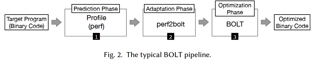
- BOLT takes as input a linked binary program
- BOLT also takes a file containing profile data as input.
- This profile data is then transformed into BOLT’s input format through an adaptation phase (using the perf2bolt tool).
- With both the input binary and the properly formatted profile data, BOLT then performs a series of optimizations to the binary.
- In practice, the most effective optimizations applied by BOLT are basic-block and function reordering, which greatly reduce CPU front-end stalls [Panchenko et al. 2019].
VESPA’s usage can be divided into two parts: "Training" and "Prediction"
- The goal of the training phase is to build an accurate prediction function.
- Training starts with feature extraction.
- Features are mined(开采)from the target program syntax.
- 提取特征后,它们会被排列成一个特征向量(Once features are extracted, they are arranged into a feature vector)
- Said vector is passed to a łpredictionž function.
- 将此函数应用到特征向量上得到的值就是发生分支的概率。(The value that results from applying this function onto the feature vector is the probability that a branch is taken.)
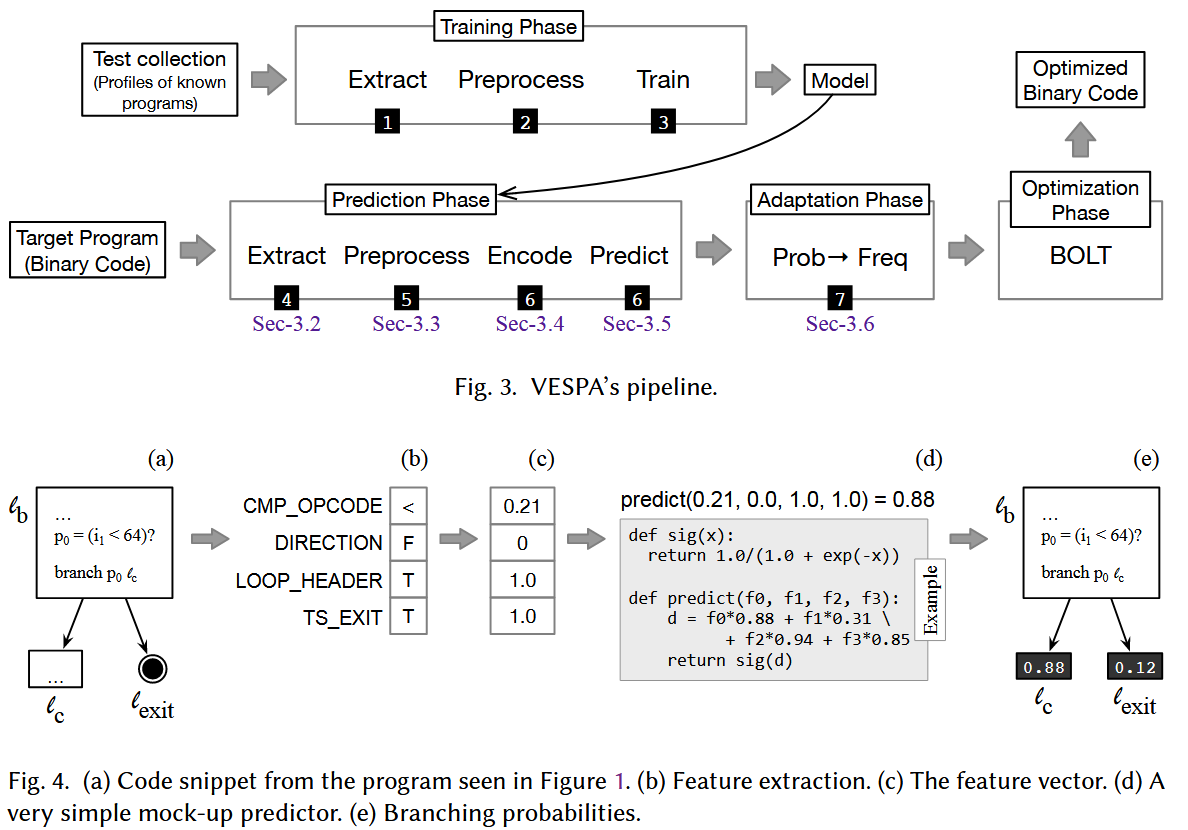
- Prediction starts with feature extraction.
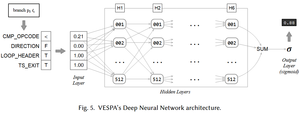
Feature Extraction
Consider the instruction \(branch \ p_0 \ l_{exit}\)
- A first feature is the opcode used to implement this instruction, e.g., in x86’s machine code: jne, je, jg, jle, jl, and jge.
- 来自一份工作:Still in the 1980’s, further improvements have been proposed on top of BTFNT, like considering the branch’s opcode [Smith 1981]
- A second feature is the opcode used to produce the value p0.
- A third feature is the direction of the branch: forward or backward.
feature 来源:
(1) The feature was originally proposed by Calder et al. [1997].
(2) The feature was proposed by Namolaru et al. [2010]. This work includes, for instance, the number of load and store instructions in the targets of branches.
(3) The feature emerged during discussions with the original engineers that worked in the BOLT project. The DELTA_TAKEN feature, for instance, came out of these discussions.
(4) The feature was thought out by the authors of this paper.
选择feature的标准
(1) It was easy to extract from the program’s binary representation.
(2) It could reduce prediction error in at least one of the benchmarks available in the test set.
(3) We could explain, at least intuitively, why the feature would lead to certain branch results.
Table 1. Categorical branch features proposed by Calder et al., and reused in this work.
| ID | Feature | Description |
|---|---|---|
| 1 | OPCODE | the opcode of the branch instruction |
| 2 | CMP_OPCODE | the opcode of the predicate operation |
| 3 | FS_END_OPCODE | the opcode of the terminal instruction in the fallthrough successor basic block |
| 4 | TS_END_OPCODE | the opcode of the terminal instruction in the taken successor basic block |
| 5 | DIRECTION | whether the branch is backward or forward (i.e. if it flows to an earlier or later address in the program’s layout) |
| 6 | LOOP_HEADER | whether the basic block containing the branch is a loop header |
| 7 | PROCEDURE_TYPE | whether the procedure containing the basic block encompassing the branch is leaf, non-leaf or recursive |
| 8 | OPERAND_RA_TYPE | the opcode of the left hand side operand |
| 9 | OPERAND_RB_TYPE | the opcode of the right hand side operand |
| 10 | TS_DOMINATES | whether the taken successor basic block is dominated by the basic block containing the branch |
| 11 | TS_POSTDOMINATES | whether the taken successor basic block post-dominates the basic block containing the branch |
| 12 | TS_LOOP_HEADER | whether the taken successor basic block is a loop header |
| 13 | TS_BACKEDGE | whether the taken successor basic block is a back edge |
| 14 | TS_EXIT | whether the taken successor basic block contains a call to exit the program |
| 15 | TS_CALL | whether the taken successor basic block contains a procedure call |
| 16 | FS_DOMINATES | whether the fallthrough successor basic block is dominated by the basic block containing the branch |
| 17 | FS_POSTDOMINATES | whether the fallthrough successor basic block post-dominates the basic block containing the branch |
| 18 | FS_LOOP_HEADER | whether the fallthrough successor basic block is a loop header |
| 19 | FS_BACKEDGE | whether the fallthrough successor basic block is a back edge |
| 20 | FS_EXIT | whether the fallthrough successor basic block contains a call to exit the program |
| 21 | FS_CALL | whether the fallthrough successor basic block contains a procedure call |
- 指令自身特征(Features 1–4)
- 控制流方向与结构(Features 5–7)
- 操作数类型(Features 8–9)
- Taken 与 Fall-through 路径特征(Features 10–21)
- 支路跳转(Taken)和不跳转(Fall-through)
new features:
-
Some of our new features try to measure the łsemantic weightž of the destination of a branch. This metric measures how heavy on different types of instructions is the basic block that is the target of a branch. Features 22-26, 52, 39-50, in Tables 2 and 3, estimate this weight.
- “语义重量”(semantic weight)特征
- 目的:量化“跳转目标基本块”里指令的“消耗”或“重要性”。
- 思路:不同指令对处理器的压力和语义意义不同——例如:
- 算术/逻辑指令(
ADD,AND等)开销较小,控制流预测意义一般; - 内存访问指令(
LOAD,STORE)可能引发缓存未命中,延迟较高; - 过程调用(
CALL)会改变调用栈,还要保存上下文; - 系统调用、退出(
EXIT,SYSCALL)则是“重”操作。
- 算术/逻辑指令(
- “语义重量”(semantic weight)特征
-
A second category of new features refers to the function that contains the branch. These features include characteristics of the function, such as the number of outermost loops that it contains (29), or the maximum depth of any loop nest (51).
- 包含分支的函数级特征
- 外层循环数(number of outermost loops):函数里有多少个彼此不嵌套的顶层
for/while循环。 - 最大循环嵌套深度(max loop nesting depth):整个函数内,从最外层到最深层的嵌套层数。
- 直观理解:
- 函数“循环密集度”:
- 外层循环多,但不深:代表函数可能在多条独立的循环上各自迭代;
- 嵌套深度高:代表有“多重嵌套”结构,某些路径会被多次迭代,分支行为更具周期性。
- 函数“循环密集度”:
- 外层循环数(number of outermost loops):函数里有多少个彼此不嵌套的顶层
- 包含分支的函数级特征
-
Finally, features 53-55 encode structural characteristics of the basic block that contains the branch.
- 包含分支的基本块结构特征(这类特征关注“该分支所在的基本块(BB)在程序结构中扮演了什么角色”)
- 是否为某个循环的退出点
- 包含分支的基本块结构特征(这类特征关注“该分支所在的基本块(BB)在程序结构中扮演了什么角色”)
Feature Preprocessing
-
The first step consists of dealing with incomplete data.
-
There may be branches for which there is insufficient data available in the disassembled binary to determine their static properties.
-
Usual culprits for incompleteness are indirect jumps. (Why?)
-
直接分支 vs. 间接分支
- 直接分支(如
jmp 0x400610、je label)的目标地址是固定常量,在反汇编里可以直接读出来。 - 间接分支(如
jmp rax、call [rip+0x200]、ret、switch语句编译后的跳表),目标取决于运行时寄存器或内存的值,反汇编阶段通常看不到它到底会跳向哪些基本块。
反汇编器的局限
- 如果反汇编器只是做线性扫描或简单递归遍历,它遇到间接跳转时可能就“断链”──无法追踪到所有可能的目标基本块。
- 结果是在 CFG 里,这条间接跳转的“后继”(successors)列表就不完整或为空。
- 直接分支(如
-
-
due to the layout of the disassembled binary, in some cases it may be difficult to track which instruction computes the predicate that controls a branch.
- 在静态反汇编时,不仅要把分支指令本身找到,还要追溯“是哪条指令”给它提供了判断条件(predicate),但有时候二进制里指令排列、编译器优化或者 flag/寄存器的多次复用,会让这种“反向数据流追踪”变得困难。具体来说:
- 什么是“控制分支的谓词(predicate)”?
- 对于一个条件分支指令(比如 x86 的
je、jl、ARM 的b.eq等),它跳不跳的依据是「某个比较/逻辑计算」的结果(CPU flag 或某条指令的输出)。 - 在编译后的二进制里,这个比较可能是一个单独的
cmp/test指令,也可能是一个算术、逻辑指令(sub、and)的一部分。
- 对于一个条件分支指令(比如 x86 的
- 为什么有时难以“追溯”到那条比较指令?
- 编译器优化:编译器可能会把比较和算术合并,或者为了流水线代价更好地重排指令顺序,使得原本“先 cmp 再 jmp”的结构被打乱。
- flag/寄存器复用:一个寄存器或标志位(carry、zero 等)可能被多次写入,分支指令要用到的那次写入可能已经被下一条指令覆盖,静态分析就不知道到底是哪次写的。
- 复杂控制流:函数内的宏、内联、switch-jump-table 这类间接跳转,或者编译器插入的检查点,都可能让“从分支往上找 cmp”变成“穿过几个看不见的中间点”,难以匹配。
- 什么是“控制分支的谓词(predicate)”?
- 在静态反汇编时,不仅要把分支指令本身找到,还要追溯“是哪条指令”给它提供了判断条件(predicate),但有时候二进制里指令排列、编译器优化或者 flag/寄存器的多次复用,会让这种“反向数据流追踪”变得困难。具体来说:
-
-
Incompleteness occurs for a small amount of branches.
-
In face of incomplete information, the missing values are replaced by default values. These defaults are the values most likely to occur in practice.
Feature Encoding
- handle categorical data
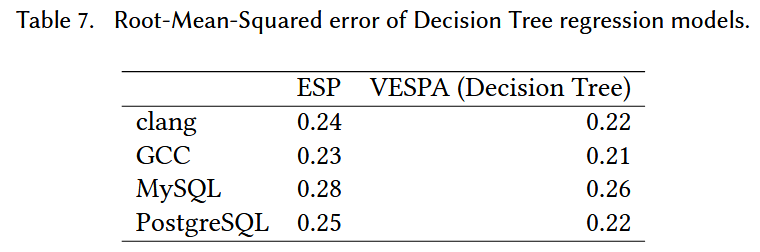
The Machine Learning Models
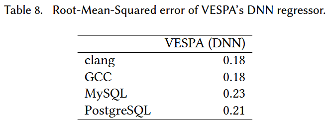
- DNN
- Dealing with Low-Frequency Branches.
- Feature Selection.
From Probabilities To Execution Frequencie
-
BOLT performs optimizations based on absolute branch counts (execution frequencies), which is the information provided by perf.
-
To map probabilities to frequencies, we resort to Wu and Larus [1994]’s method.
-
For implementing VESPA’s step to convert probabilities into execution frequencies: implement it directly within BOLT.
-
Therefore, we implemented this step as an alternative execution mode in BOLT, which can be enabled by a command-line option. When this option is used, BOLT attempts to read the input profile data from a .pdata probabilities file, rather than the usual .fdata file produced by perf2bolt. Moreover, we also added two extra flags to BOLT to control whether to convert probabilities into absolute counts using the interprocedural or intraprocedural algorithms proposed by Wu and Larus.(因此,我们将此步骤实现为 BOLT 中的替代执行模式,可以通过命令行选项启用。使用此选项时,BOLT 会尝试从 .pdata 概率文件而不是 perf2bolt 生成的通常的 .fdata 文件读取输入配置文件数据。此外,我们还为 BOLT 添加了两个额外的标志,以控制是否使用 Wu 和 Larus 提出的过程间或过程内算法将概率转换为绝对计数。)
-
Thus, for the sake of practicality, given these inherent imprecisions, validation allows for a deviation of up to 20% between incoming and outgoing frequencies.
EVALUATION
实验环境:
-
CPU: Intel Xeon E5-2620 CPU at 2.00GHz
-
Memory: 16GB RAM
-
OS: Linux Ubuntu 18.04, kernel version 4.15.0-123
-
BOLT version: commit 8028b7b
-
perf version: Linux’s perf, version 4.15.18
DNN的训练集和测试集来源:
-
To train our model, we used the eleven programs in SPEC CINT2006 plus 226 programs from the LLVM test-suite, for which we collected execution profiles using instrumentation.
-
训练集:We have used 80% of the branches from these programs to train the prediction model.
-
测试集:Of the remaining branches, half were used to test the model and the other half to validate it (for tuning purposes).
-
only 513,316 branches were associated with profile information.
既然训练时的labs为CFG中basic block branch执行的次数(频率),那么DNN输出应该也可以是一个预测的频率数值哇
为什么这里作者要将DNN输出的值硬搞成概率?
难道labs为执行branch的概率?
测试模型的数据集:
• The clang compiler, version 7, as used in BOLT’s reference tutorial [Panchenko 2018], compiling its own source code as input;
• The GCC compiler, version 7, compiling clang 7’s source code as input.
• The MySQL database management system, version 8.0, with the oltp_point_select benchmark from the SysBench3 suite as input.
• The PostgreSQL database management system, version 13.2, with the select-only benchmark from the PgBench4 suite as input.
原因:
- BOLT’s optimization effects can only be perceived once the hot parts of a program are too large to fit into the instruction cache. (BOLT的优化效果只有在程序的热部分太大而无法适合指令缓存才显著)
Experimental Methodology:
实验方法:本节报告的运行时间均为十次独立执行的平均值。我们对比优化前后性能时,均使用 Student’s t 检验来检验原假设——“无论采用静态剖析还是动态剖析对二进制进行优化,都不会引起性能变化”——在 95% 置信水平下,所有试验的 P 值均小于 0.05。
比较方法:
-
baseline: compiled using clang 12 (at -O3)
-
VESPA
-
BOLT Dynamic profile
-
...
与原方法(Calder et al.)比较预测精确度:
- 比较方法:使用本论文提出的新feature和原feature训练出来的模型相比
- 指标为 branch probabilities
- 顺便与本文改进的DNN相比:
与使用各个static profiling/dynamic profiling投喂BOLT 然后比较性能提升:
- GCC和clang的性能指标为execution time speedup.
- MySQL和PostgreSQL的性能指标为throughput, 即the number of Transactions Per Seconds (TPS)
- baseline: built with clang -O3.
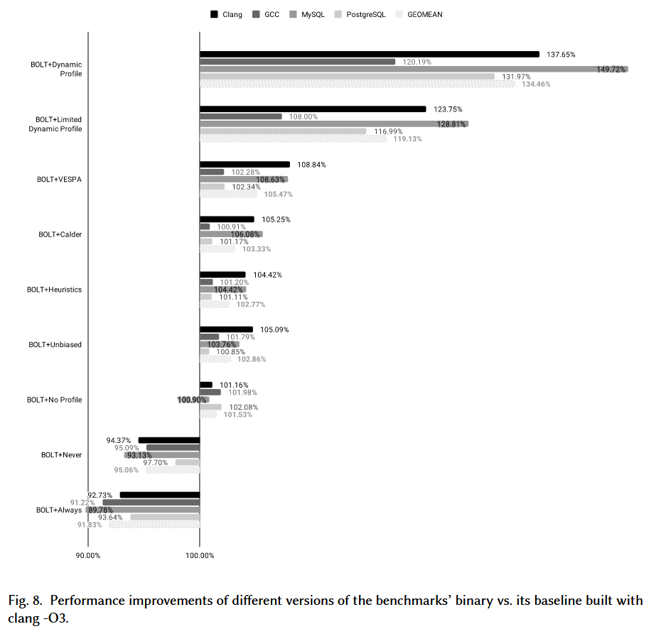
BOLT + Dynamic: 与 clang -O3 相比,整体性能提高了 34.46%(几何平均值)
然而,一旦删除间接跳转的动态分析信息,这一优势就会下降到 19.13%。(静态配置文件均不涉及间接分支,因此我们认为这是一个更好的比较点。)
使用 VESPA 生成的配置文件优化的二进制文件在静态分析启发式方法中产生了最佳结果。
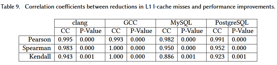
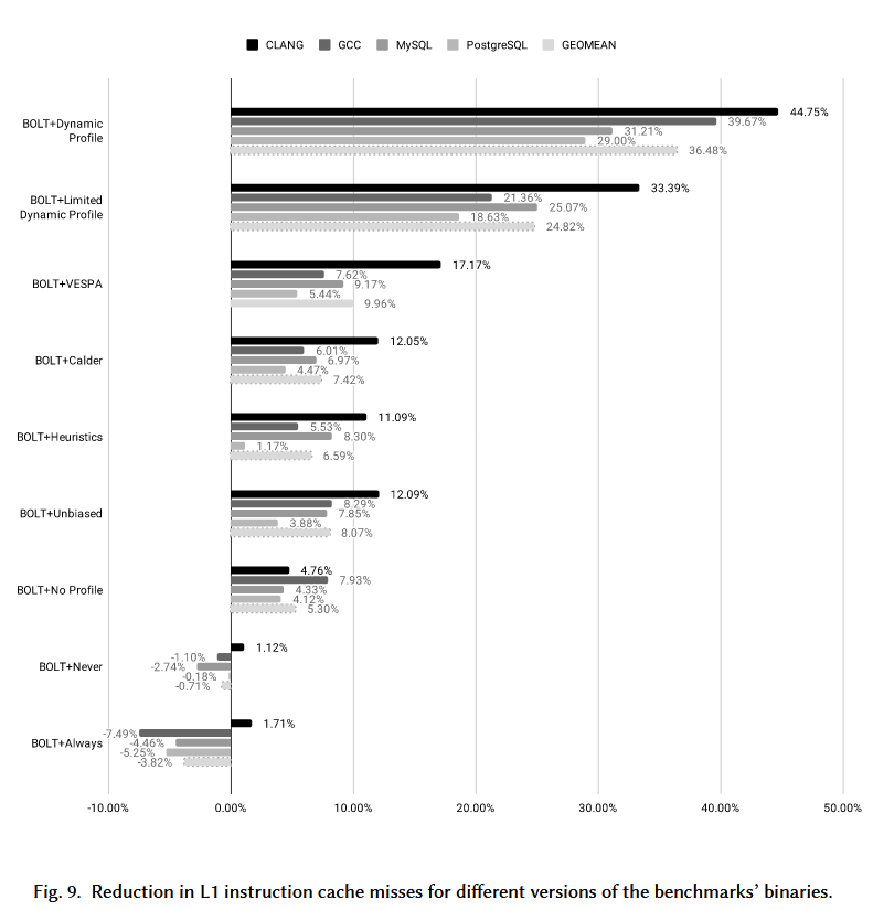
比较在L1 I-cache miss上的提升:
比较生成优化后的二进制代码的时间:
- When timing BOLT with the dynamic profiler, we count the time to
- run the target application to collect samples
- plus the time to run BOLT to disassemble and optimize the binary.
- In the case of VESPA, we measured:
- (i) the time to run BOLT to disassemble and collect static features;
- (ii) the time to run the predictor to generate a static profile;
- (iii) the time to run BOLT again, this time fed with the static profile information.
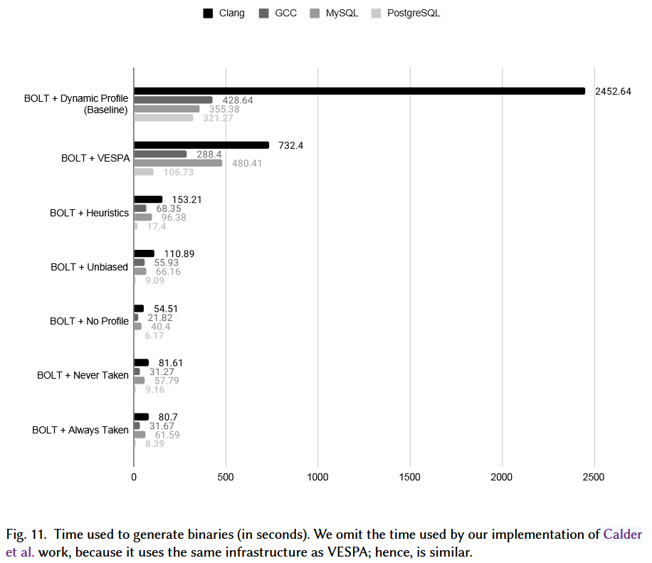
However, for the MySQL binary, BOLT with a dynamic profile is actually faster, by a factor of about 30%. This is due to the relatively short running time of MySQL’s profiling inputs, which allows for fast sampling. In contrast, VESPA spends time not only running the predictor, but also importing them and embedding them onto the program’s binary representation.
Nevertheless, we emphasize that in cases where VESPA takes longer to generate a binary, this overhead is constant.(尽管如此,我们强调,在 VESPA 花费更长时间生成二进制文件的情况下,这种开销是恒定的。)
RELATED WORK
Hardware-Based Branch Prediction
All the approaches mentioned in this paper, including BOLT guided by dynamic profiling, perform predictions offline; that is, before the program runs.
Hardware-based methods, in turn, do it online, i.e., while the program is running. Online techniques use dynamic information to carry out branch prediction. This information is stored in hardware-based tables such as the Local History Register (LHR), the Global History Register (GHR), and the Global Addresses Map (GA).
This dynamic data can be used to feed regression and classification models. Such possibilities have been demonstrated by previous work [Kalla et al. 2017; Mao et al. 2018; Tarsa et al. 2019].

 浙公网安备 33010602011771号