动手学深度学习_4 多层感知机

多层感知机原理
隐藏层
严格一点来讲:我们需要隐藏层是因为线性是一个很强的假设,线性模型在有些情况会不适用或者出错。
- 一个形象的例子:
就如同上面图片中展示的XOR问题,如果我们现在想要将绿和红球分开,如果只用一条"线性",我们会发现我们是做不到的,起码要两条及以上的"线性"

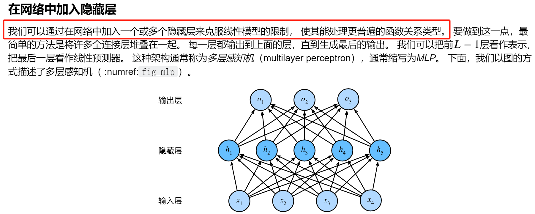
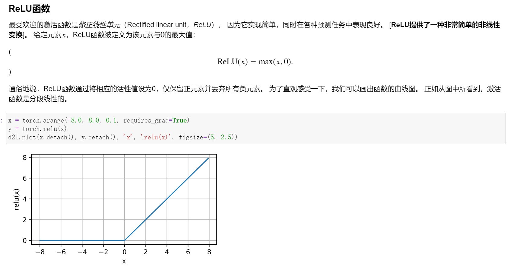
激活函数
简单来说激活函数的作用是将隐藏层的输出从线性转换为非线性
一般来说,有了激活函数,就不可能再将我们的多层感知机退化成线性模型
多层感知机的从零开始实现
import torch
from torch import nn
from d2l import torch as d2l
from IPython import display


# 可视化
class Accumulator:  #@save
    """在n个变量上累加"""
    def __init__(self, n):
        self.data = [0.0] * n

    def add(self, *args):
        self.data = [a + float(b) for a, b in zip(self.data, args)]

    def reset(self):
        self.data = [0.0] * len(self.data)

    def __getitem__(self, idx):
        return self.data[idx]

def accuracy(y_hat, y):  #@save
    """计算预测正确的数量"""
    if len(y_hat.shape) > 1 and y_hat.shape[1] > 1:
        y_hat = y_hat.argmax(axis=1)
    cmp = y_hat.type(y.dtype) == y
    return float(cmp.type(y.dtype).sum())

def evaluate_accuracy(net, data_iter):  #@save
    """计算在指定数据集上模型的精度"""
    if isinstance(net, torch.nn.Module):
        net.eval()  # 将模型设置为评估模式
    metric = Accumulator(2)  # 正确预测数、预测总数
    with torch.no_grad():
        for X, y in data_iter:
            metric.add(accuracy(net(X), y), y.numel())
    return metric[0] / metric[1]


class Animator:  #@save
    """在动画中绘制数据"""
    def __init__(self, xlabel=None, ylabel=None, legend=None, xlim=None,
                 ylim=None, xscale='linear', yscale='linear',
                 fmts=('-', 'm--', 'g-.', 'r:'), nrows=1, ncols=1,
                 figsize=(3.5, 2.5)):
        # 增量地绘制多条线
        if legend is None:
            legend = []
        d2l.use_svg_display()
        self.fig, self.axes = d2l.plt.subplots(nrows, ncols, figsize=figsize)
        if nrows * ncols == 1:
            self.axes = [self.axes, ]
        # 使用lambda函数捕获参数
        self.config_axes = lambda: d2l.set_axes(
            self.axes[0], xlabel, ylabel, xlim, ylim, xscale, yscale, legend)
        self.X, self.Y, self.fmts = None, None, fmts

    def add(self, x, y):
        # 向图表中添加多个数据点
        if not hasattr(y, "__len__"):
            y = [y]
        n = len(y)
        if not hasattr(x, "__len__"):
            x = [x] * n
        if not self.X:
            self.X = [[] for _ in range(n)]
        if not self.Y:
            self.Y = [[] for _ in range(n)]
        for i, (a, b) in enumerate(zip(x, y)):
            if a is not None and b is not None:
                self.X[i].append(a)
                self.Y[i].append(b)
        self.axes[0].cla()
        for x, y, fmt in zip(self.X, self.Y, self.fmts):
            self.axes[0].plot(x, y, fmt)
        self.config_axes()
        display.display(self.fig)
        display.clear_output(wait=True)

# 训练
def train_epoch_ch3(net, train_iter, loss, updater):  #@save
    """训练模型一个迭代周期(定义见第3章)"""
    # 将模型设置为训练模式
    if isinstance(net, torch.nn.Module):
        net.train()
    # 训练损失总和、训练准确度总和、样本数
    metric = Accumulator(3)
    for X, y in train_iter:
        # 计算梯度并更新参数
        y_hat = net(X) # X.shape:torch.Size([256, 1, 28, 28]),y_hat得到的是一个256x10的矩阵
        l = loss(y_hat, y) #y.shape:torch.Size([256]),l.shape:torch.Size([256])
        if isinstance(updater, torch.optim.Optimizer):
            # 使用PyTorch内置的优化器和损失函数
            updater.zero_grad()
            l.mean().backward()
            updater.step()
        else:
            # 使用定制的优化器和损失函数
            l.sum().backward()
            updater(X.shape[0])
        metric.add(float(l.sum()), accuracy(y_hat, y), y.numel())
    # 返回训练损失和训练精度
    return metric[0] / metric[2], metric[1] / metric[2]

def train_ch3(net, train_iter, test_iter, loss, num_epochs, updater):  #@save
    """训练模型(定义见第3章)"""
    animator = Animator(xlabel='epoch', xlim=[1, num_epochs], ylim=[0.3, 0.9],
                        legend=['train loss', 'train acc', 'test acc'])
    for epoch in range(num_epochs):
        train_metrics = train_epoch_ch3(net, train_iter, loss, updater)
        test_acc = evaluate_accuracy(net, test_iter)
        animator.add(epoch + 1, train_metrics + (test_acc,))
    train_loss, train_acc = train_metrics
    assert train_loss < 0.5, train_loss
    assert train_acc <= 1 and train_acc > 0.7, train_acc
    assert test_acc <= 1 and test_acc > 0.7, test_acc


#获取数据
batch_size = 256
train_iter, test_iter = d2l.load_data_fashion_mnist(batch_size)

#初始化模型参数
num_inputs, num_outputs, num_hiddens = 784, 10, 256

W1 = nn.Parameter(torch.randn(
    num_hiddens,num_inputs ,requires_grad=True) * 0.01)
b1 = nn.Parameter(torch.zeros(num_hiddens, requires_grad=True))
W2 = nn.Parameter(torch.randn(
    num_outputs,num_hiddens ,requires_grad=True) * 0.01)
b2 = nn.Parameter(torch.zeros(num_outputs, requires_grad=True))

params = [W1, b1, W2, b2]

# 定义激活函数
def relu(X):
    # torch.zeros_like是一个模仿X的shape但是将其中元素全部填充为0
    a = torch.zeros_like(X)
    return torch.max(X, a)

# 定义模型
def net(X):
    # 这里X一来照样是X.shape:torch.Size([256, 1, 28, 28])
    # 然后通过下面的操作变成[256,784]
    X = X.reshape((-1, num_inputs))
    # b是一个向量,W1我设置的是256x784 这里要转置一下,X@W1.t()为256x256
    H = relu(X@W1.t() + b1)  # 这里“@”代表矩阵乘法
    return (H@W2.t() + b2)

# 定义损失函数
loss = nn.CrossEntropyLoss(reduction='none')

# 定义优化函数
num_epochs, lr = 10, 0.1
updater = torch.optim.SGD(params, lr=lr)

# 训练
train_ch3(net, train_iter, test_iter, loss, num_epochs, updater)
模型选择、欠拟合和过拟合
模型选择
在机器学习中,我们通常在评估几个候选模型后选择最终的模型。 这个过程叫做模型选择。
- 进行比较的模型在本质上是完全不同的(比如,决策树与线性模型)
- 比较不同的超参数设置下的同一类模型
在我们确定所有的超参数之前,我们不希望用到测试集,我们决不能依靠测试数据进行模型选择.(即我们不能通过测试集进行训练来进行调整参数,我们只能通过测试集进行判断最终哪个模型的好坏)
在实际应用中,情况变得更加复杂。 虽然理想情况下我们只会使用测试数据一次, 以评估最好的模型或比较一些模型效果,但现实是测试数据很少在使用一次后被丢弃。 我们很少能有充足的数据来对每一轮实验采用全新测试集。
于是我们可以在训练数据较少的情况下使用𝐾折交叉验证
欠拟合和过拟合
代码:
import math
import numpy as np
import torch
from torch import nn
from d2l import torch as d2l


# 可视化
class Accumulator:  #@save
    """在n个变量上累加"""
    def __init__(self, n):
        self.data = [0.0] * n

    def add(self, *args):
        self.data = [a + float(b) for a, b in zip(self.data, args)]

    def reset(self):
        self.data = [0.0] * len(self.data)

    def __getitem__(self, idx):
        return self.data[idx]

def accuracy(y_hat, y):  #@save
    """计算预测正确的数量"""
    if len(y_hat.shape) > 1 and y_hat.shape[1] > 1:
        y_hat = y_hat.argmax(axis=1)
    cmp = y_hat.type(y.dtype) == y
    return float(cmp.type(y.dtype).sum())

def evaluate_accuracy(net, data_iter):  #@save
    """计算在指定数据集上模型的精度"""
    if isinstance(net, torch.nn.Module):
        net.eval()  # 将模型设置为评估模式
    metric = Accumulator(2)  # 正确预测数、预测总数
    with torch.no_grad():
        for X, y in data_iter:
            metric.add(accuracy(net(X), y), y.numel())
    return metric[0] / metric[1]


class Animator:  #@save
    """在动画中绘制数据"""
    def __init__(self, xlabel=None, ylabel=None, legend=None, xlim=None,
                 ylim=None, xscale='linear', yscale='linear',
                 fmts=('-', 'm--', 'g-.', 'r:'), nrows=1, ncols=1,
                 figsize=(3.5, 2.5)):
        # 增量地绘制多条线
        if legend is None:
            legend = []
        d2l.use_svg_display()
        self.fig, self.axes = d2l.plt.subplots(nrows, ncols, figsize=figsize)
        if nrows * ncols == 1:
            self.axes = [self.axes, ]
        # 使用lambda函数捕获参数
        self.config_axes = lambda: d2l.set_axes(
            self.axes[0], xlabel, ylabel, xlim, ylim, xscale, yscale, legend)
        self.X, self.Y, self.fmts = None, None, fmts

    def add(self, x, y):
        # 向图表中添加多个数据点
        if not hasattr(y, "__len__"):
            y = [y]
        n = len(y)
        if not hasattr(x, "__len__"):
            x = [x] * n
        if not self.X:
            self.X = [[] for _ in range(n)]
        if not self.Y:
            self.Y = [[] for _ in range(n)]
        for i, (a, b) in enumerate(zip(x, y)):
            if a is not None and b is not None:
                self.X[i].append(a)
                self.Y[i].append(b)
        self.axes[0].cla()
        for x, y, fmt in zip(self.X, self.Y, self.fmts):
            self.axes[0].plot(x, y, fmt)
        self.config_axes()
        display.display(self.fig)
        display.clear_output(wait=True)

# 训练
def train_epoch_ch3(net, train_iter, loss, updater):  #@save
    """训练模型一个迭代周期(定义见第3章)"""
    # 将模型设置为训练模式
    if isinstance(net, torch.nn.Module):
        net.train()
    # 训练损失总和、训练准确度总和、样本数
    metric = Accumulator(3)
    for X, y in train_iter:
        # 计算梯度并更新参数
        y_hat = net(X) # X.shape:torch.Size([256, 1, 28, 28]),y_hat得到的是一个256x10的矩阵
        l = loss(y_hat, y) #y.shape:torch.Size([256]),l.shape:torch.Size([256])
        if isinstance(updater, torch.optim.Optimizer):
            # 使用PyTorch内置的优化器和损失函数
            updater.zero_grad()
            l.mean().backward()
            updater.step()
        else:
            # 使用定制的优化器和损失函数
            l.sum().backward()
            updater(X.shape[0])
        metric.add(float(l.sum()), accuracy(y_hat, y), y.numel())
    # 返回训练损失和训练精度
    return metric[0] / metric[2], metric[1] / metric[2]


# 准备数据
max_degree = 20  # 多项式的最大阶数
n_train, n_test = 100, 100  # 训练和测试数据集大小
true_w = np.zeros(max_degree)  # 分配大量的空间
# 20x1
true_w[0:4] = np.array([5, 1.2, -3.4, 5.6])

# 这里是在生成数据集X 200x1
features = np.random.normal(size=(n_train + n_test, 1))

#np.random.shuffle(features)是一个用于随机打乱NumPy数组或列表features元素顺序的操作。
#这个函数会在原地修改features数组,重新排列其中的元素,使其以随机顺序出现。
np.random.shuffle(features)

# np.power(features, np.arange(max_degree).reshape(1, -1))将原始特征features的每个元素分别提升到对应次数的幂,
# 根据上面生成的次数数组来计算。结果是一个矩阵,其中每一行包含了原始特征的不同次幂。
# 原来是200x1,然后对于每一个xi,都形成xi^0,xi^1....xi^19,即是每一行包含了原始特征的不同次幂。所以形成了200x20
# poly_features 200x20
poly_features = np.power(features, np.arange(max_degree).reshape(1, -1))

# 这里是将每一个(x)i)^i 变成 (x)i)^i / i!
for i in range(max_degree):
    poly_features[:, i] /= math.gamma(i + 1)  # gamma(n)=(n-1)!
# labels的维度:(n_train+n_test,),这里labels是真实的y,是用于跟我们模型得到的结果进行比较用的
#200x1
labels = np.dot(poly_features, true_w)
labels += np.random.normal(scale=0.1, size=labels.shape)
# NumPy ndarray转换为tensor
true_w, features, poly_features, labels = [torch.tensor(x, dtype=
    torch.float32) for x in [true_w, features, poly_features, labels]]


# 定义损失评估函数
def evaluate_loss(net, data_iter, loss):  #@save
    """评估给定数据集上模型的损失"""
    metric = d2l.Accumulator(2)  # 损失的总和,样本数量
    for X, y in data_iter:
        out = net(X)
        y = y.reshape(out.shape)
        l = loss(out, y)
        metric.add(l.sum(), l.numel())
    return metric[0] / metric[1]

# 训练
def train(train_features, test_features, train_labels, test_labels,
          num_epochs=400):
    loss = nn.MSELoss(reduction='none')
    input_shape = train_features.shape[-1]
    # 不设置偏置,因为我们已经在多项式中实现了它
    net = nn.Sequential(nn.Linear(input_shape, 1, bias=False))
    batch_size = min(10, train_labels.shape[0])
    train_iter = d2l.load_array((train_features, train_labels.reshape(-1,1)),
                                batch_size)
    test_iter = d2l.load_array((test_features, test_labels.reshape(-1,1)),
                               batch_size, is_train=False)
    trainer = torch.optim.SGD(net.parameters(), lr=0.01)
    animator = d2l.Animator(xlabel='epoch', ylabel='loss', yscale='log',
                            xlim=[1, num_epochs], ylim=[1e-3, 1e2],
                            legend=['train', 'test'])
    for epoch in range(num_epochs):
        train_epoch_ch3(net, train_iter, loss, trainer)
        if epoch == 0 or (epoch + 1) % 20 == 0:
            animator.add(epoch + 1, (evaluate_loss(net, train_iter, loss),
                                     evaluate_loss(net, test_iter, loss)))
    print('weight:', net[0].weight.data.numpy())


# 从多项式特征中选择前4个维度,即1,x,x^2/2!,x^3/3!
# poly_features[:n_train, :4] 这是一种切片的写法,表示提取出poly_features中0~n_train-1行0~3列的内容
# 正常
train(poly_features[:n_train, :4], poly_features[n_train:, :4],
      labels[:n_train], labels[n_train:])


# 从多项式特征中选择前2个维度,即1和x
# 欠拟合
train(poly_features[:n_train, :2], poly_features[n_train:, :2],
      labels[:n_train], labels[n_train:])

# 从多项式特征中选取所有维度
# 过拟合
train(poly_features[:n_train, :], poly_features[n_train:, :],
      labels[:n_train], labels[n_train:], num_epochs=1500)
权重衰退
正则化处理过拟合问题
回想一下上面过拟合问题的出现原因:
模型容量太大,而数据过简单
所谓的模型容量与模型复杂度,模型中x的个数有关
在解决过拟合的问题中,在训练集的损失函数中加入惩罚项,以降低学习到的模型的复杂度。这是一种方法,其通过限制w的范围从而达到避免模型向着过于复杂的函数去拟合
如上图所示,蓝线呈现的波动较大的函数可以理解为是损失函数中没有加入惩罚项,可以看到即使在数据集上的数据都拟合上了,但是其余地方拟合的过于复杂
绿线呈现的波动较小的函数可以理解为损失函数中加入惩罚项后,惩罚项起作用了,模型在拟合的时候没有这么复杂
那么惩罚项到底是如何工作的呢?
权重衰退原理
权重衰减(weight decay)是最广泛使用的正则化的技术之一, 它通常也被称为 𝐿2正则化。 这项技术通过函数与零的距离来衡量函数的复杂度。 因为在所有函数 𝑓中,函数 𝑓=0(所有输入都得到值 0) 在某种意义上是最简单的。
如何衡量函数与零的距离?
一种简单的方法是通过线性函数 𝑓(𝐱)=𝐰⊤𝐱 中的权重向量的某个范数来度量其复杂性, 例如 ‖𝐰‖2。
要保证权重向量比较小, 最常用方法是将其范数作为惩罚项加到最小化损失的问题中。为何这种方法可以呢?原因如下:
将原来的训练目标最小化训练标签上的预测损失, 调整为最小化预测损失和惩罚项之和。 现在,如果我们的权重向量增长的太大, 我们的学习算法可能会更集中于最小化权重范数 ‖𝐰‖2。 这正是我们想要的。

- 此外,为什么我们首先使用 𝐿2范数,而不是 𝐿1范数?
- 使用 𝐿2范数的一个原因是它对权重向量的大分量施加了巨大的惩罚。 这使得我们的学习算法偏向于在大量特征上均匀分布权重的模型。
- 在实践中,这可能使它们对单个变量中的观测误差更为稳定。相比之下, 𝐿1惩罚会导致模型将权重集中在一小部分特征上, 而将其他权重清除为零。 这称为特征选择(feature selection),这可能是其他场景下需要的。
代码实现
%matplotlib inline
import torch
from torch import nn
from d2l import torch as d2l

# 获取数据
# 每一个数据都是有num_inputs个输入(即有200个feature(即x))
n_train, n_test, num_inputs, batch_size = 20, 100, 200, 5
true_w, true_b = torch.ones((num_inputs, 1)) * 0.01, 0.05

# 总的训练数据集中数据个数为n_train个(每一个数据都是包含X,y)
train_data = d2l.synthetic_data(true_w, true_b, n_train)
# 生成数据迭代器,每一次迭代器返回batch_size个数据
train_iter = d2l.load_array(train_data, batch_size)

# 总的训练数据集中数据个数为n_test个,
test_data = d2l.synthetic_data(true_w, true_b, n_test)
# 生成数据迭代器,每一次迭代器返回batch_size个数据
test_iter = d2l.load_array(test_data, batch_size, is_train=False)

# 初始化参数
def init_params():
    # w 200x1
    w = torch.normal(0, 1, size=(num_inputs, 1), requires_grad=True)
    # b 为向量大小为1
    b = torch.zeros(1, requires_grad=True)
    return [w, b]

# 定义惩罚项
def l2_penalty(w):
    return torch.sum(w.pow(2)) / 2

# 训练
def train(lambd):
    w, b = init_params()
    # 创建匿名函数,接受参数X
    net, loss = lambda X: d2l.linreg(X, w, b), d2l.squared_loss

    # 训练100次,学习度为0.003
    num_epochs, lr = 100, 0.003

    # 可视化
    animator = d2l.Animator(xlabel='epochs', ylabel='loss', yscale='log',
                            xlim=[5, num_epochs], legend=['train', 'test'])

    for epoch in range(num_epochs):

        for X, y in train_iter:
            # 增加了L2范数惩罚项,
            # 广播机制使l2_penalty(w)成为一个长度为batch_size的向量
            # lambd是公式中的入,为超参数
            l = loss(net(X), y) + lambd * l2_penalty(w)
            l.sum().backward()
            d2l.sgd([w, b], lr, batch_size)
        if (epoch + 1) % 5 == 0:
            animator.add(epoch + 1, (d2l.evaluate_loss(net, train_iter, loss),
                                     d2l.evaluate_loss(net, test_iter, loss)))
    print('w的L2范数是:', torch.norm(w).item())


# [忽略正则化直接训练]
train(lambd=0)
# [使用权重衰减]
train(lambd=3)
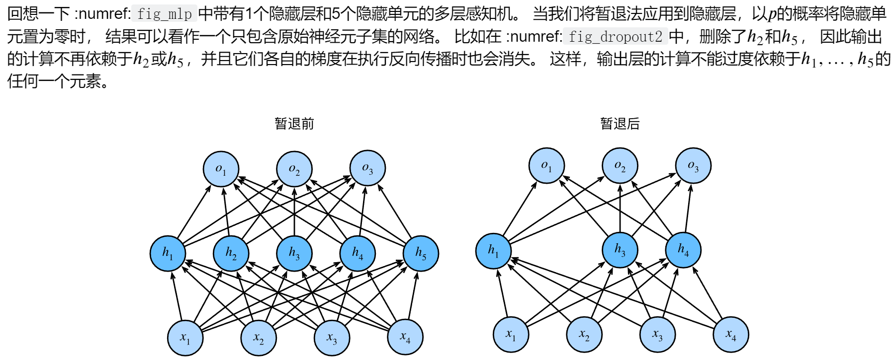
暂退法(丢弃法)
暂退法(丢弃法)原理
- 为何需要暂退法(丢弃法)?
定义一下什么是一个“好”的预测模型?
我们期待“好”的预测模型能在未知的数据上有很好的表现
为了缩小训练和测试性能之间的差距,应该以简单的模型为目标
1.简单性以较小维度的形式展现
2.简单性的另一个角度是平滑性,即函数不应该对其输入的微小变化敏感。
在训练过程中,他们建议在计算后续层之前向网络的每一层注入噪声。 因为当训练一个有多层的深层网络时,注入噪声只会在输入-输出映射上增强平滑性。这个想法被称为暂退法(dropout)。
简单来说,暂退法是用来提高模型的泛化性,即可以减缓过拟合问题,方法就是在深度神经网络中的隐藏层中加入噪音
- 如何加入噪音?
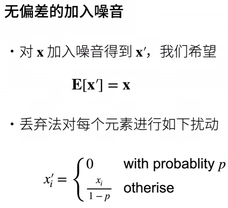
上述公式在实践的过程中给人的感觉就是在隐藏层中有些神经元有一定概率“消失”(即xi'=0),有些神经元有一定概率权重变大(即xi/(1-p),因为0<=p<1,所以xi'会变大)

需要注意的是:一般为了保证结果的稳定性,我们只在训练的时候使用dropout,在测试的时候不使用
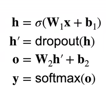
我们在使用完激活函数后进行dropout
- 对于超参数的选择
dropout中的p这个概率是个超参数,一般的选择方法是在较浅的隐藏层中p选择较小,即隐藏层的神经单元更不容易消失,随着越深p也变的越大
代码实现
import torch
from torch import nn
from IPython import display
from d2l import torch as d2l

# 可视化
class Accumulator:  #@save
    """在n个变量上累加"""
    def __init__(self, n):
        self.data = [0.0] * n

    def add(self, *args):
        self.data = [a + float(b) for a, b in zip(self.data, args)]

    def reset(self):
        self.data = [0.0] * len(self.data)

    def __getitem__(self, idx):
        return self.data[idx]

def accuracy(y_hat, y):  #@save
    """计算预测正确的数量"""
    if len(y_hat.shape) > 1 and y_hat.shape[1] > 1:
        y_hat = y_hat.argmax(axis=1)
    cmp = y_hat.type(y.dtype) == y
    return float(cmp.type(y.dtype).sum())

def evaluate_accuracy(net, data_iter):  #@save
    """计算在指定数据集上模型的精度"""
    if isinstance(net, torch.nn.Module):
        net.eval()  # 将模型设置为评估模式
    metric = Accumulator(2)  # 正确预测数、预测总数
    with torch.no_grad():
        for X, y in data_iter:
            metric.add(accuracy(net(X), y), y.numel())
    return metric[0] / metric[1]


class Animator:  #@save
    """在动画中绘制数据"""
    def __init__(self, xlabel=None, ylabel=None, legend=None, xlim=None,
                 ylim=None, xscale='linear', yscale='linear',
                 fmts=('-', 'm--', 'g-.', 'r:'), nrows=1, ncols=1,
                 figsize=(3.5, 2.5)):
        # 增量地绘制多条线
        if legend is None:
            legend = []
        d2l.use_svg_display()
        self.fig, self.axes = d2l.plt.subplots(nrows, ncols, figsize=figsize)
        if nrows * ncols == 1:
            self.axes = [self.axes, ]
        # 使用lambda函数捕获参数
        self.config_axes = lambda: d2l.set_axes(
            self.axes[0], xlabel, ylabel, xlim, ylim, xscale, yscale, legend)
        self.X, self.Y, self.fmts = None, None, fmts

    def add(self, x, y):
        # 向图表中添加多个数据点
        if not hasattr(y, "__len__"):
            y = [y]
        n = len(y)
        if not hasattr(x, "__len__"):
            x = [x] * n
        if not self.X:
            self.X = [[] for _ in range(n)]
        if not self.Y:
            self.Y = [[] for _ in range(n)]
        for i, (a, b) in enumerate(zip(x, y)):
            if a is not None and b is not None:
                self.X[i].append(a)
                self.Y[i].append(b)
        self.axes[0].cla()
        for x, y, fmt in zip(self.X, self.Y, self.fmts):
            self.axes[0].plot(x, y, fmt)
        self.config_axes()
        display.display(self.fig)
        display.clear_output(wait=True)

# 训练
def train_epoch_ch3(net, train_iter, loss, updater):  #@save
    """训练模型一个迭代周期(定义见第3章)"""
    # 将模型设置为训练模式
    if isinstance(net, torch.nn.Module):
        net.train()
    # 训练损失总和、训练准确度总和、样本数
    metric = Accumulator(3)
    for X, y in train_iter:
        # 计算梯度并更新参数
        y_hat = net(X) # X.shape:torch.Size([256, 1, 28, 28]),y_hat得到的是一个256x10的矩阵
        l = loss(y_hat, y) #y.shape:torch.Size([256]),l.shape:torch.Size([256])
        if isinstance(updater, torch.optim.Optimizer):
            # 使用PyTorch内置的优化器和损失函数
            updater.zero_grad()
            l.mean().backward()
            updater.step()
        else:
            # 使用定制的优化器和损失函数
            l.sum().backward()
            updater(X.shape[0])
        metric.add(float(l.sum()), accuracy(y_hat, y), y.numel())
    # 返回训练损失和训练精度
    return metric[0] / metric[2], metric[1] / metric[2]

def train_ch3(net, train_iter, test_iter, loss, num_epochs, updater):  #@save
    """训练模型(定义见第3章)"""
    animator = Animator(xlabel='epoch', xlim=[1, num_epochs], ylim=[0.3, 0.9],
                        legend=['train loss', 'train acc', 'test acc'])
    for epoch in range(num_epochs):
        train_metrics = train_epoch_ch3(net, train_iter, loss, updater)
        test_acc = evaluate_accuracy(net, test_iter)
        animator.add(epoch + 1, train_metrics + (test_acc,))
    train_loss, train_acc = train_metrics
    assert train_loss < 0.5, train_loss
    assert train_acc <= 1 and train_acc > 0.7, train_acc
    assert test_acc <= 1 and test_acc > 0.7, test_acc


# 定义dropout函数
def dropout_layer(X, dropout):
    assert 0 <= dropout <= 1
    # 在本情况中,所有元素都被丢弃
    if dropout == 1:
        return torch.zeros_like(X)
    # 在本情况中,所有元素都被保留
    if dropout == 0:
        return X
    #这里mask是与X形状相同的01矩阵
    mask = (torch.rand(X.shape) > dropout).float()
    #mask*X是矩阵中每一个相同位置处的元素相乘,得到的还是原来形状大小的矩阵
    return mask * X / (1.0 - dropout)


# 获取数据
# 一次feature有784个,label有10个,第一层隐藏层神经元个数为256个,第二层隐藏层神经元个数为256个
num_inputs, num_outputs, num_hiddens1, num_hiddens2 = 784, 10, 256, 256
num_epochs,batch_size = 10,256
train_iter, test_iter = d2l.load_data_fashion_mnist(batch_size)

# 定义模型参数
lr=0.5

# 定义模型
dropout1, dropout2 = 0.2, 0.5

class Net(nn.Module):
    def __init__(self, num_inputs, num_outputs, num_hiddens1, num_hiddens2,
                 is_training = True):
        super(Net, self).__init__()
        self.num_inputs = num_inputs
        self.training = is_training
        self.lin1 = nn.Linear(num_inputs, num_hiddens1)
        self.lin2 = nn.Linear(num_hiddens1, num_hiddens2)
        self.lin3 = nn.Linear(num_hiddens2, num_outputs)
        # 激活函数:
        self.relu = nn.ReLU()

    def forward(self, X):
        H1 = self.relu(self.lin1(X.reshape((-1, self.num_inputs))))
        # 只有在训练模型时才使用dropout
        if self.training == True:
            # 在第一个全连接层之后添加一个dropout层
            H1 = dropout_layer(H1, dropout1)
        H2 = self.relu(self.lin2(H1))
        if self.training == True:
            # 在第二个全连接层之后添加一个dropout层
            H2 = dropout_layer(H2, dropout2)
        out = self.lin3(H2)
        return out

net = Net(num_inputs, num_outputs, num_hiddens1, num_hiddens2)

# 定义损失函数
loss = nn.CrossEntropyLoss(reduction='none')

# 定义优化函数
trainer = torch.optim.SGD(net.parameters(), lr=lr)

# 训练
train_ch3(net, train_iter, test_iter, loss, num_epochs, trainer)
数值稳定性和模型初始化
数值稳定的两大问题
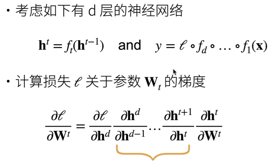
我们的梯度如果不进行一定的限制,那么当很多层梯度都十分大或者都十分小的时候,就会导致梯度爆炸或者梯度消失
-
梯度爆炸
参数更新过大,破坏了模型的稳定收敛

-
梯度消失
参数更新过小,在每次更新时几乎不会移动,导致模型无法学习

模型初始化
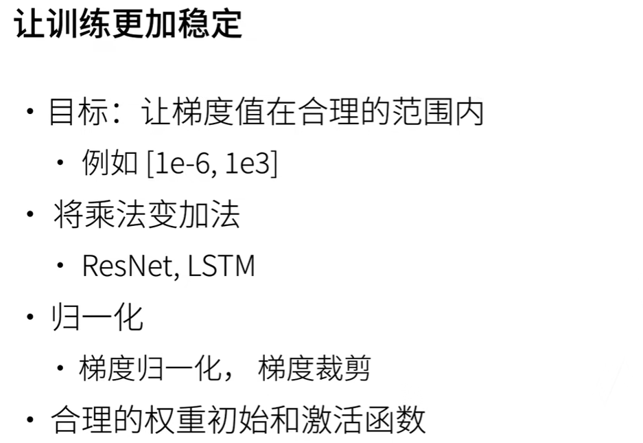
这里我们重点讲的是如何进行合理的权重初始和激活函数
权重初始的依据原理
现在以我们的多层感知机为例,进行如下假设:
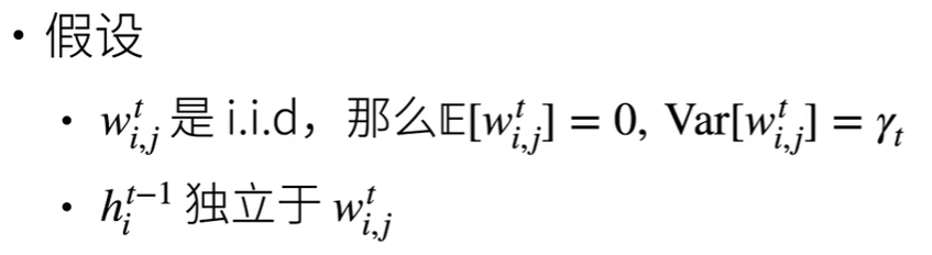
i.i.d是独立同分布的意思
这里我们是假设均值和方差分布为0与yt
这里的w来解释一下:上标t表示第t层隐藏层,下标i,j分别表示第i个神经元输出中第j个输入的权重
这里的h来解释一下:上标t表示第t层隐藏层,下标i表示第i个神经元输出
现在再假设我们没有激活函数(即在计算的时候不使用激活函数)
于是上述公式我们学过概率统计应该很简单推导出来
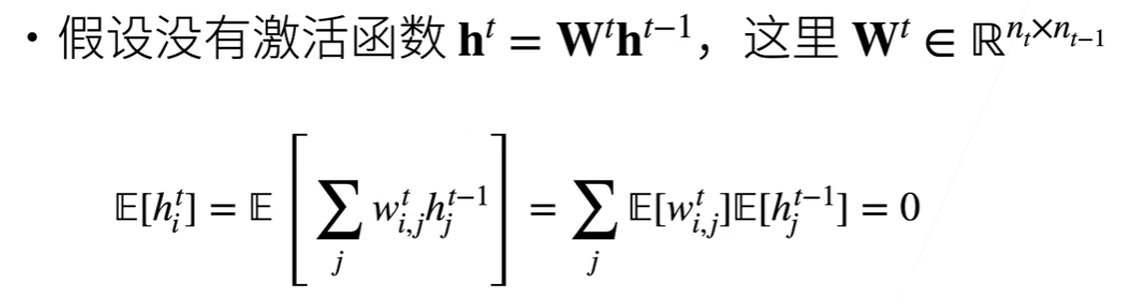
均值计算完了,下面我们再来计算一下正向传播时的方差:
这里解释下n: 因为我们假设每一个上标为t的w的方差都为yt,那么

再结合公式这里的求和符号,我们可以得到其实nt-1表示第t-1层隐藏层中神经元的个数(即第t层隐藏层的输入个数)
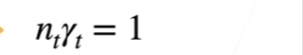
如果我们想要避免梯度爆炸或者是梯度消失,最好是保持着隐藏层中各个输出的方差不变最好,即

算完正向我们再来看看反向计算是的均值与方差(因为我们要反向传播计算梯度)
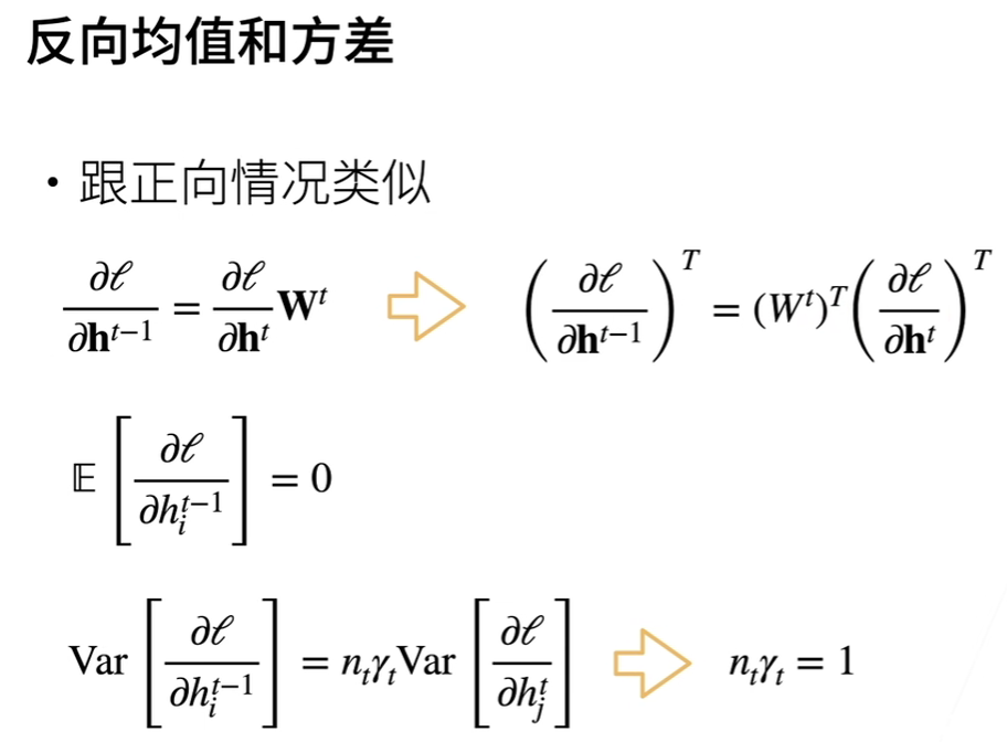
这里我们也是希望在反向计算的时候,输出的方差最好不会有变化,推到:
权重初始
根据上述原理可以指导我们在对各个隐藏层的权重进行初始化时应该如何做:
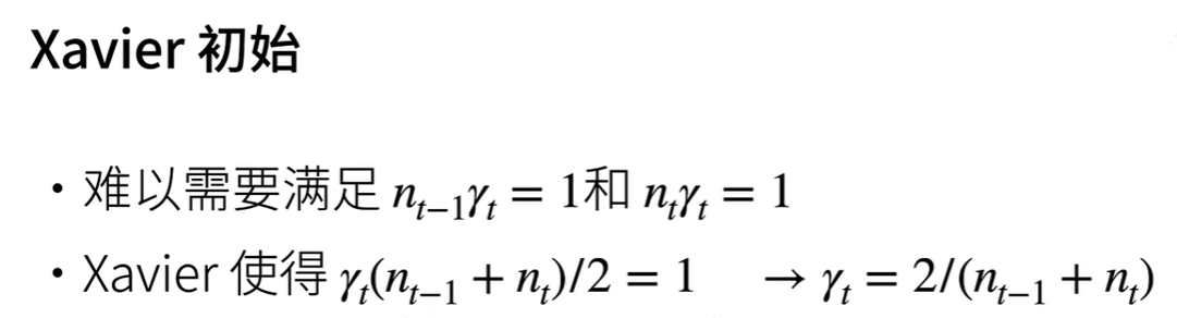
因为每一层隐藏层的神经元个数(输入个数)我们是可以推导出来的,所以上述初始化是可以实现的
激活函数的选择原理
因为上述假设我们是假设没有激活函数的,现在我们加上激活函数
为了理论推导的方便,这里我们的激活函数是线性的(实际上我们是不会用线性激活函数的,这里只是为了理论推导的方便)
同样为了数值稳定,我希望输出的均值和方差都不变
那么就推导到了α=1,β=0,那不就说明我们的激活函数只要不是f(x)=x都会导致均值和方差的变化吗?
激活函数的选择
画出图来可以发现,因为一般我们的激活函数也就是将数值拉到0~1这个范围出,而恰好我们的聚会函数在x为 0~1 这个范围内与f(x)=x这个函数十分相近,这也就是为何我们的激活函数在实践中有效的原因
Kaggle 房价预测实战
𝐾折交叉验证
代码实现
最基础的书上代码实现:
import torch
from torch import nn
import matplotlib.pyplot as plt
import numpy as np
from torch.utils import data
import pandas as pd
# 首先要下载数据
# 到官网上下载训练数据和测试数据:https://www.kaggle.com/competitions/house-prices-advanced-regression-techniques/data
# 下载完成保存到本地的D:\pythonProject\AIStudy\Kaggle
traindata_name = 'D:\pythonProject\AIStudy\Kaggle\\train.csv'
testdata_name = 'D:\pythonProject\AIStudy\Kaggle\\test.csv'
# train_data 1460x81 ; test_data=1459x80
train_data = pd.read_csv(traindata_name)
test_data = pd.read_csv(testdata_name)
# print(train_data.shape)
# print(test_data.shape)

# 预处理数据
# 肯定是train_data和test_data一起处理,所以先将他们合并在一起,id 没啥用去除,train_data的最后一列是label要另存
# all_features 2919x79
all_features = pd.concat((train_data.iloc[:, 1:-1], test_data.iloc[:, 1:]))
# print (all_features.shape)


# 处理数值数据
# 消除不同特征数据之间的尺度差距,处理方法是x=(x-u)/σ
numeric_features = all_features.dtypes[all_features.dtypes != 'object'].index
for col in numeric_features:
    all_features[col] = (all_features[col] - all_features[col].mean()) / all_features[col].std()
# print (f'{numeric_features}\n')
# 处理空缺值
# 上述处理完后,要处理数值数据中的空缺值,因为我们已经将尺度消除,可以将空缺值直接设置为0
all_features[numeric_features] = all_features[numeric_features].fillna(0)

# 然后再处理非数值数据
# 将其作为特征来看待
# all_features 2919x330
all_features = pd.get_dummies(all_features, dummy_na=True)
all_features = all_features.astype(float)
# print (all_features.shape)
# print (all_features.iloc[0:4,[0,1,2,3,-3,-2,-1]])

# 获取数据
# 数据全部预处理完毕后提取出我们真正要训练和预测的数据
n_train = train_data.shape[0]  # n_train是原先训练集数据有多少个
# train_features 1460x331
train_features = torch.tensor(all_features[:n_train].values, dtype=torch.float32)
# train_labels 1460x1
train_labels = torch.tensor(train_data.SalePrice.values.reshape(-1, 1), dtype=torch.float32)
# print(train_features.shape,train_labels.shape)
test_features = torch.tensor(all_features[n_train:].values, dtype=torch.float32)


def load_array(data_arrays, batch_size, is_train=True):
    """构造一个PyTorch数据迭代器"""
    dataset = data.TensorDataset(*data_arrays)
    return data.DataLoader(dataset, batch_size, shuffle=is_train)


# 定义模型
def get_net():
    return nn.Sequential(nn.Linear(train_features.shape[1], 1))


# 定义损失函数
# 可能这里面会自动根据输入的X的数据个数进行计算损失值,我在外面使用的时候就不用管这些了,
# 只要定义一次每一次训练的时候用多少数据(batch_size)就行
loss = nn.MSELoss()


# 我们也要对损失值进行消除尺度影响,我们在训练的时候还是用loss,
# 但是我们在观看损失结果的时候为了避免某些尺度较大的损失值可能会导致损失结果不能真正反应出学习的效果
# 方法是将sqrt((∑(logy_hat-logy)^2)/n)
def log_rmse(net, features, labels):
    clipped_preds = torch.clamp(net(features), 1, float('inf'))
    rmse = torch.sqrt(loss(torch.log(clipped_preds), torch.log(labels)))
    return rmse.item()


# 定义优化函数 与 训练
def train(net, train_features, train_labels, test_features, test_labels,
          num_epochs, learning_rate, weight_decay, batch_size):
    train_ls, test_ls = [], []
    # 获取数据迭代器
    train_iter = load_array([train_features, train_labels], batch_size)
    # 获取优化函数
    # 这里使用的是Adam优化算法,Adam是优化算法,其利用梯度下降更新w与b这些参数
    # 这里模型参数是在net.parameters()中了
    # weight_decay 是使用权重衰减中超参数,用来衡量L2范式的权重
    optimizer = torch.optim.Adam(net.parameters(),
                                 lr=learning_rate,
                                 weight_decay=weight_decay)
    # 总共训练num_epochs次
    for epoch in range(num_epochs):
        # 每一次训练取出batch_size个数据进行训练
        for X, y in train_iter:
            # 去除原来的梯度
            optimizer.zero_grad()
            l = loss(net(X), y)
            l.backward()
            # 进行反向传播,进行梯度下降对参数更新
            optimizer.step()
        # 用更新后的权重看下训练的效果(均方误差)
        # 注意这里是用全部的训练组数据进行计算
        train_ls.append(log_rmse(net, train_features, train_labels))
        if (test_labels is not None):
            # 用更新后的权重看下预测的效果(如果这次训练有测试组的话)
            test_ls.append(log_rmse(net, test_features, test_labels))
    return train_ls, test_ls


# 获得K折交叉验证数据
def get_k_fold_data(k, i, X, y):
    assert k > 1
    fold_size = X.shape[0] // k
    train_fs, train_ls, test_fs, test_ls = None, None, None, None
    for j in range(k):
        X_part = X[j * fold_size:(j + 1) * fold_size, :]
        y_part = y[j * fold_size:(j + 1) * fold_size]
        if j == i:
            test_fs = X_part
            test_ls = y_part
        elif train_fs is None:
            train_fs = X_part
            train_ls = y_part
        else:
            train_fs = torch.cat([train_fs, X_part], 0)
            train_ls = torch.cat([train_ls, y_part], 0)
    return train_fs, train_ls, test_fs, test_ls


# 使用K折交叉验证
def k_fold(k, X_train, y_train, num_epochs, learning_rate, weight_decay, batch_size):
    train_ls_sum, test_ls_sum = 0, 0
    # 每一个选择第i+1组作为测试组,其余组作为训练组
    for i in range(k):
        # 获得测试组和训练组的数据
        data = get_k_fold_data(k, i, X_train, y_train)
        # 得到各个训练次数时,训练组和测试组的损失值
        train_ls, test_ls = train(get_net(), *data, num_epochs, learning_rate, weight_decay, batch_size)
        # 只画出当i==0时的训练损失变化图
        if i == 0:
            x = range(num_epochs)
            plt.plot(x, train_ls, label='Train Data', color='blue')
            plt.plot(x, test_ls, label='Test Data', color='red', linestyle='--')
            plt.xlabel('epochs')
            plt.ylabel('loss')
        # 为计算最终K折全部训练完成后的平均损失值而求和
        train_ls_sum += train_ls[-1]
        test_ls_sum += test_ls[-1]
        # 打印出各个i时的最终训练损失
        print(f'折{i + 1},训练log rmse{float(train_ls[-1]):f}, '
              f'验证log rmse{float(test_ls[-1]):f}')
    return train_ls_sum / k, test_ls_sum / k


# 定义模型参数
# 这里w,b之类的参数不用我们自己定义我们有nn.parameters()
k, num_epochs, lr, weight_decay, batch_size = 5, 100, 5, 0, 64
train_l, test_l = k_fold(k, train_features, train_labels, num_epochs, lr, weight_decay, batch_size)
print(f'{k}-折验证: 平均训练log rmse: {float(train_l):f}, '
      f'平均验证log rmse: {float(test_l):f}')


# 进行预测
# test_features变量在这里终于排上用场了,test_features是我们最后要预测的数据,最初始的数据是test_data
# 我们经过数据预处理后就成了test_features了
def train_and_pred(train_features, train_labels, test_features, test_data,
                   num_epochs, lr, weight_decay, batch_size):
    net = get_net()
    # 将全部的训练数据拿过来进行最后一次训练
    train_ls, _ = train(net, train_features, train_labels, None, None, num_epochs, lr, weight_decay, batch_size)
    print(f'训练log rmse:{float(train_ls[-1]):f}')
    # 画出图来
    plt.figure(2)
    x = range(num_epochs)
    plt.plot(x, train_ls, label='Train Data', color='blue')
    plt.xlabel('epochs')
    plt.ylabel('loss')
    # 然后进行预测
    # 最后只要用我们训练完成的net进行预测即可,train中的一大堆东西都是为了梯度下降得到较好的w与b而已
    preds = net(test_features).detach().numpy()
    # 打包要提交的数据
    test_data['SalePrice'] = pd.Series(preds.reshape(1, -1)[0])
    submission = pd.concat([test_data['Id'], test_data['SalePrice']], axis=1)
    submission.to_csv('submission.csv', index=False)


train_and_pred(train_features,  train_labels, test_features,test_data, num_epochs, lr, weight_decay, batch_size)
下面用了多层感知机和防止过拟合的方法(但是效果实在太差了)
主要是改动了定义模型和定义模型参数那里
import torch
from torch import nn
import matplotlib.pyplot as plt
import numpy as np
from torch.utils import data
import pandas as pd
# 首先要下载数据
# 到官网上下载训练数据和测试数据:https://www.kaggle.com/competitions/house-prices-advanced-regression-techniques/data
# 下载完成保存到本地的D:\pythonProject\AIStudy\Kaggle
traindata_name = 'D:\pythonProject\AIStudy\Kaggle\\train.csv'
testdata_name = 'D:\pythonProject\AIStudy\Kaggle\\test.csv'
# train_data 1460x81 ; test_data=1459x80
train_data = pd.read_csv(traindata_name)
test_data = pd.read_csv(testdata_name)
# print(train_data.shape)
# print(test_data.shape)

# 预处理数据
# 肯定是train_data和test_data一起处理,所以先将他们合并在一起,id 没啥用去除,train_data的最后一列是label要另存
# all_features 2919x79
all_features = pd.concat((train_data.iloc[:, 1:-1], test_data.iloc[:, 1:]))
# print (all_features.shape)


# 处理数值数据
# 消除不同特征数据之间的尺度差距,处理方法是x=(x-u)/σ
numeric_features = all_features.dtypes[all_features.dtypes != 'object'].index
for col in numeric_features:
    all_features[col] = (all_features[col] - all_features[col].mean()) / all_features[col].std()
# print (f'{numeric_features}\n')
# 处理空缺值
# 上述处理完后,要处理数值数据中的空缺值,因为我们已经将尺度消除,可以将空缺值直接设置为0
all_features[numeric_features] = all_features[numeric_features].fillna(0)

# 然后再处理非数值数据
# 将其作为特征来看待
# all_features 2919x330
all_features = pd.get_dummies(all_features, dummy_na=True)
all_features = all_features.astype(float)
# print (all_features.shape)
# print (all_features.iloc[0:4,[0,1,2,3,-3,-2,-1]])

# 获取数据
# 数据全部预处理完毕后提取出我们真正要训练和预测的数据
n_train = train_data.shape[0]  # n_train是原先训练集数据有多少个
# train_features 1460x331
train_features = torch.tensor(all_features[:n_train].values, dtype=torch.float32)
# train_labels 1460x1
train_labels = torch.tensor(train_data.SalePrice.values.reshape(-1, 1), dtype=torch.float32)
# print(train_features.shape,train_labels.shape)
test_features = torch.tensor(all_features[n_train:].values, dtype=torch.float32)


def load_array(data_arrays, batch_size, is_train=True):
    """构造一个PyTorch数据迭代器"""
    dataset = data.TensorDataset(*data_arrays)
    return data.DataLoader(dataset, batch_size, shuffle=is_train)


# 定义模型 与 模型参数
dropout1=0.15
num_inputs, num_outputs, num_hiddens1= train_features.shape[1], 1, 85
k, num_epochs, lr, weight_decay, batch_size = 5, 85, 4.5, 0.05, 115
def get_net():
    # train_features.shape[1] 为331
    net = nn.Sequential(nn.Flatten(),
        nn.Linear(num_inputs, num_hiddens1),
        nn.ReLU(),
        # 在第一个全连接层之后添加一个dropout层
        nn.Dropout(dropout1),
        nn.Linear(num_hiddens1,num_outputs))
    return net


# 定义损失函数
# 可能这里面会自动根据输入的X的数据个数进行计算损失值,我在外面使用的时候就不用管这些了,
# 只要定义一次每一次训练的时候用多少数据(batch_size)就行
loss = nn.MSELoss()


# 我们也要对损失值进行消除尺度影响,我们在训练的时候还是用loss,
# 但是我们在观看损失结果的时候为了避免某些尺度较大的损失值可能会导致损失结果不能真正反应出学习的效果
# 方法是将sqrt((∑(logy_hat-logy)^2)/n)
def log_rmse(net, features, labels):
    clipped_preds = torch.clamp(net(features), 1, float('inf'))
    rmse = torch.sqrt(loss(torch.log(clipped_preds), torch.log(labels)))
    return rmse.item()


# 定义优化函数 与 定义训练函数
def train(net, train_features, train_labels, test_features, test_labels,
          num_epochs, learning_rate, weight_decay, batch_size):
    train_ls, test_ls = [], []
    # 获取数据迭代器
    train_iter = load_array([train_features, train_labels], batch_size)
    # 获取优化函数
    # 这里使用的是Adam优化算法,Adam是优化算法,其利用梯度下降更新w与b这些参数
    # 这里模型参数是在net.parameters()中了
    # weight_decay 是使用权重衰减中超参数,用来衡量L2范式的权重
    optimizer = torch.optim.Adam(net.parameters(),
                                 lr=learning_rate,
                                 weight_decay=weight_decay)
    # 总共训练num_epochs次
    for epoch in range(num_epochs):
        # 每一次训练取出batch_size个数据进行训练
        for X, y in train_iter:
            # 去除原来的梯度
            optimizer.zero_grad()
            l = loss(net(X), y)
            l.backward()
            # 进行反向传播,进行梯度下降对参数更新
            optimizer.step()
        # 用更新后的权重看下训练的效果(均方误差)
        # 注意这里是用全部的训练组数据进行计算
        train_ls.append(log_rmse(net, train_features, train_labels))
        if (test_labels is not None):
            # 用更新后的权重看下预测的效果(如果这次训练有测试组的话)
            test_ls.append(log_rmse(net, test_features, test_labels))
    return train_ls, test_ls


# 获得K折交叉验证数据
def get_k_fold_data(k, i, X, y):
    assert k > 1
    fold_size = X.shape[0] // k
    train_fs, train_ls, test_fs, test_ls = None, None, None, None
    for j in range(k):
        X_part = X[j * fold_size:(j + 1) * fold_size, :]
        y_part = y[j * fold_size:(j + 1) * fold_size]
        if j == i:
            test_fs = X_part
            test_ls = y_part
        elif train_fs is None:
            train_fs = X_part
            train_ls = y_part
        else:
            train_fs = torch.cat([train_fs, X_part], 0)
            train_ls = torch.cat([train_ls, y_part], 0)
    return train_fs, train_ls, test_fs, test_ls


# 使用K折交叉验证
def k_fold(k, X_train, y_train, num_epochs, learning_rate, weight_decay, batch_size):
    train_ls_sum, test_ls_sum = 0, 0
    # 每一个选择第i+1组作为测试组,其余组作为训练组
    for i in range(k):
        # 获得测试组和训练组的数据
        data = get_k_fold_data(k, i, X_train, y_train)
        # 得到各个训练次数时,训练组和测试组的损失值
        train_ls, test_ls = train(get_net(), *data, num_epochs, learning_rate, weight_decay, batch_size)
        # 只画出当i==0时的训练损失变化图
        if i == 0:
            x = range(num_epochs)
            plt.plot(x, train_ls, label='Train Data', color='blue')
            plt.plot(x, test_ls, label='Test Data', color='red', linestyle='--')
            plt.xlabel('epochs')
            plt.ylabel('loss')
        # 为计算最终K折全部训练完成后的平均损失值而求和
        train_ls_sum += train_ls[-1]
        test_ls_sum += test_ls[-1]
        # 打印出各个i时的最终训练损失
        print(f'折{i + 1},训练log rmse{float(train_ls[-1]):f}, '
              f'验证log rmse{float(test_ls[-1]):f}')
    return train_ls_sum / k, test_ls_sum / k


# 训练
# 这里w,b之类的参数不用我们自己定义我们有nn.parameters()
train_l, test_l = k_fold(k, train_features, train_labels, num_epochs, lr, weight_decay, batch_size)
print(f'{k}-折验证: 平均训练log rmse: {float(train_l):f}, '
      f'平均验证log rmse: {float(test_l):f}')


# 进行预测
# test_features变量在这里终于排上用场了,test_features是我们最后要预测的数据,最初始的数据是test_data
# 我们经过数据预处理后就成了test_features了
def train_and_pred(train_features, train_labels, test_features, test_data,
                   num_epochs, lr, weight_decay, batch_size):
    net = get_net()
    # 将全部的训练数据拿过来进行最后一次训练
    train_ls, _ = train(net, train_features, train_labels, None, None, num_epochs, lr, weight_decay, batch_size)
    print(f'训练log rmse:{float(train_ls[-1]):f}')
    # 画出图来
    plt.figure(2)
    x = range(num_epochs)
    plt.plot(x, train_ls, label='Train Data', color='blue')
    plt.xlabel('epochs')
    plt.ylabel('loss')
    # 然后进行预测
    # 最后只要用我们训练完成的net进行预测即可,train中的一大堆东西都是为了梯度下降得到较好的w与b而已
    preds = net(test_features).detach().numpy()
    # 打包要提交的数据
    test_data['SalePrice'] = pd.Series(preds.reshape(1, -1)[0])
    submission = pd.concat([test_data['Id'], test_data['SalePrice']], axis=1)
    submission.to_csv('submission4.csv', index=False)


train_and_pred(train_features,  train_labels, test_features,test_data, num_epochs, lr, weight_decay, batch_size)
数据分析
对应这个比赛数据如何预处理?
一篇行动总指南
一篇手把手教如何处理的好博文
关于Feature Engineering的,较你如何处理数据使得数据更"线性",这里有一系列教程,其中还有关于Mutual Information的教程,是一种新的衡量相关性的指标
处理分类特征的教程,教你如何处理数据中非数值的特征变量
关于Pandas的最基本用法
步骤分析
一般步骤可以归结如下:
了解预测变量和特征变量的含义
这个过程就初步给个概念
处理缺失值
对于缺失值更加实际情况可以填充,可以删除
但是不管咋样,我们先看看缺失情况才能进一步分析:
第三方库可视化
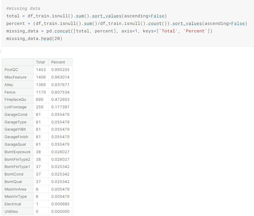
panda 计算
然后我们可以看看这些缺失特征变量之间的关系,缺失程度,与预测变量的关系,来决定是删除还是填充保留
处理分类变量
将字符串的变量转换为数值,这个操作在如下有详细教程
处理分类特征的教程,教你如何处理数据中非数值的特征变量
分析预测变量,以及特征变化和预测变量的关系
前置知识
回归的假设
即:
线性性
我们假设预测变量和特征变量的关系是线性的,可以通过绘制散点图看出是否为线性从而判断这个假设是否正确
同方差性
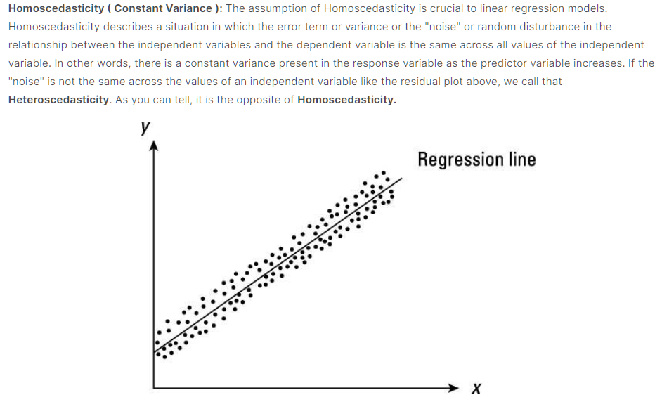
即同方差描述了一种情况,其中自变量和因变量之间的关系中的误差项或方差或“噪声”或随机扰动在自变量的所有值中都相同。
所谓误差项这个和我们的线性回归方程有关,因为在方程中误差项是固定的,所以如果对应不同自变量他们对应的因变量之间误差很大,那么我们的方程(模型)也就不准确了
比较好的情况是如上图中全部的点围绕着直线无规律分布
这个是否符合同方差性可以通过绘制散点图和残差图可以看出:
如残差图:
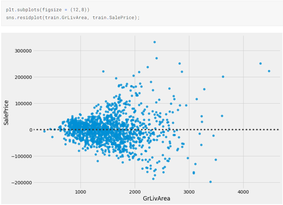
从上述图可以看到,点分布有明显规律:随着GrlivArea的值增大,残差的分布也逐渐变大
同理散点图也可以按照这个方法判断
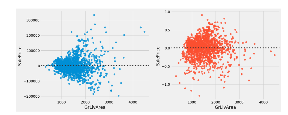
像上图右边的残差图,点的分布较无规律形成一团云状(而不像左边是漏斗状)
多元正态性
即假设我们的预测变化和特征变量都是符号正态分布的
这个可以通过绘制QQ图:
If you are learning about Q-Q-plots for the first time. checkout this video.
上述的视频讲解了为何QQ图可以反应出正态分布的特征:
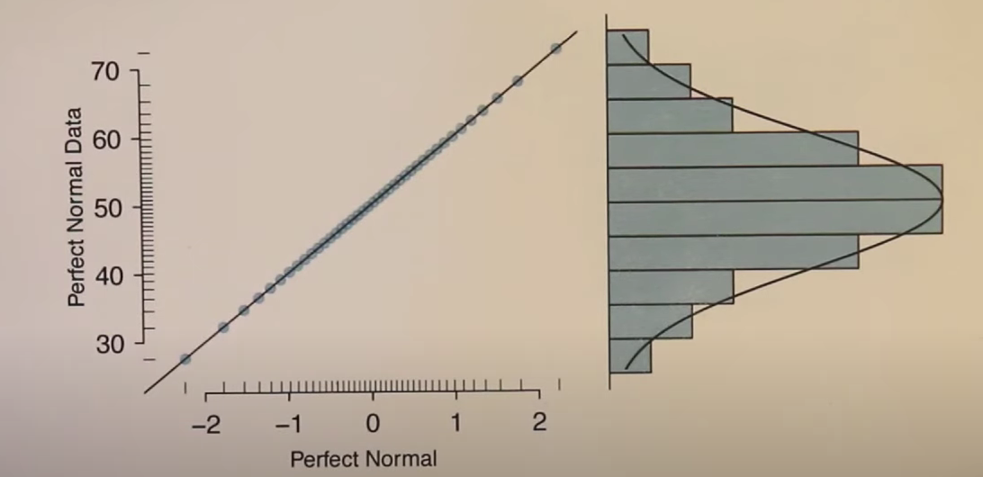
QQ图的横坐标是正态分布的值,其反应了正态分布的分布特征和数值大小
纵坐标是数据的数值,其反应了数据分布的特征和数值大小特征
上述图横纵左边都是标准的正态分布,所以"点们"呈现处理的就是直线
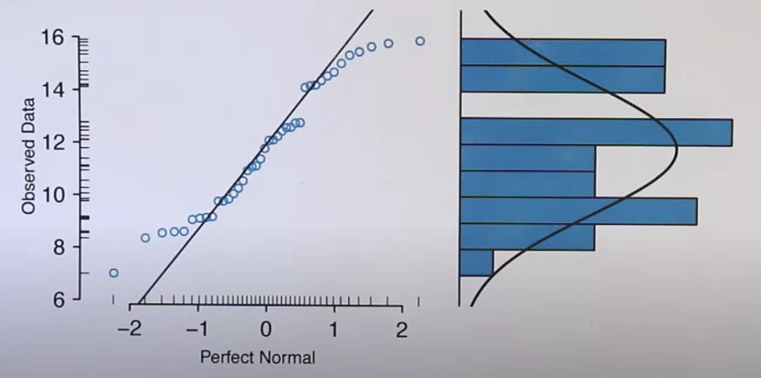
但是看看这幅图,其纵坐标展示的数据分布明显不是正态分布,所以反应到曲线上的也是与直线有区别的样子
没有或很少有多重共线问题
即假设我们的特征变量之间都是独立无关系的
但是一般我们的数据不同特征变量之间是有相关性的
多重共线性可能导致各种问题,包括:
- 我们的回归估计的预测变量的影响将取决于我们的模型中包含哪些其他变量。
- 根据样本中的观察结果,预测变量可能会产生截然不同的结果,并且样本中的微小变化可能会导致非常不同的估计效果。由于多重共线性非常高,计算机计算的逆矩阵可能不准确。
- 我们不能再将变量的系数解释为在保持其他变量不变的情况下该变量增加一单位对目标的影响。 其背后的原因是,当预测变量强相关时,不存在一个变量可以在另一个变量有条件变化的情况下发生变化的情况。
实践
通过绘制预测变量的QQ图,直方分布图和描述性统计看看预测变量是否是符合正态分布,以及分布情况
如果非正态分布,我们可以通过取log 将数据进行转化
然后再看看预测变量与特征变量的关系
通过绘制散点图,看下有无明显线性关系,是否有异常值
判断是否要删除异常值
注意!线性回归对于异常值十分敏感,需要处理
然后通过绘制热力图,看看不同特征变量之间的关系,判断是否要删除相关性较高的特征变量,从而避免违反了 没有或者较少多重共线性问题 的假设
然后我们再解决一下其他的回归假设问题
非同方差性(异方差)问题,可以通过解决非正态分布而解决,其实这些假设一般是同时出现的,一个方面解决了,另一个方面会有较大好转
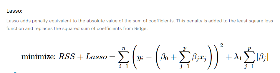
正则化
正则化是我用线性回归模型时为了避免模型太复杂而过拟合问题而提出的方法
其一般方法如下:
其方法就是在我们计算普通的误差平方和时,加入正则惩罚项
这个时候我们的目的从最小化误差平方和 变成了 最小化时在误差平方和的最小和模型复杂度最小做权衡
比如对应岭回归我们的误差函数变成了:

 浙公网安备 33010602011771号