基于拉勾网的深圳数据分析职位分析

 

　　　　　　　　　　　　　　　基于拉勾网的深圳数据分析职位分析

一、选题的背景

随着毕业生人数的上涨，如何及时获取有效就业信息并加以分析做出相应决策对于大学生而言显得尤为重要。传统的搜索招聘网站、各单位官网、人力资源网等，可以获得海量的就业信息，然而这种方式都需要到相应网站翻页查找，在不同网站之间切换，耗时、速度慢、不及时、不利于集中分析统计等缺点，导致大学生容易错过适合的岗位信息。针对这种情况，提出了基于网络爬虫的就业数据分析，为大学生搜索分析就业信息提供一定的参考价值。

 

二、主题式网络爬虫设计方案

1.主题式网络爬虫名称：

基于拉勾网的深圳数据分析职位分析

主题式网络爬虫爬取的内容与数据特征分析：

以拉勾网作为实例，对如何开发爬虫获取信息，及对获取的信息快速分析进行了深入探讨与研究。

2.

主题式网络爬虫设计方案概述（包括实现思路与技术难点）：

网络爬虫程序的开发是否成功取决于确保系统能够实现用户定制功能，达到预期设计目的。因此，在网络爬虫程序设计之前，就需要对该程序需求加以详细的分析，从而对整体的设计有一个清晰的思路。时下，普遍适用的爬虫程序都是模块化的，模块化的程序设计有利于代码块的测试与维护，而且也进一步增加了代码的适用性。在此基础上，只要对各个模块进行组合，就能够构建出一个完整的爬虫程序。

因为研究旨在通过爬虫程序对当前就业进行分析，所以需要通过编写爬虫程序抓取相关岗位的就业信息，获取的信息包括公司名称、公司规模、招聘岗位、公司福利、工作地址、薪资水平、工作经验、职位类型、学历要求、发布日期等，并将抓取的就业信息保存在数据库中，以便后期进行数据处理和可视化分析。

爬虫系统的设计思路：首先，需要获得所有包括岗位信息网页的源码；其次，在每一页的网页源码中寻找出与需求相匹配的信息，此时就需要连接爬虫系统和数据库，将每次成功匹配到的信息均存入数据库中，直至所有网页检索完毕。

 

三，结构特征分析

1，结构与特征分析

 

 

 

 

 

 

 

 

 

 

 

 

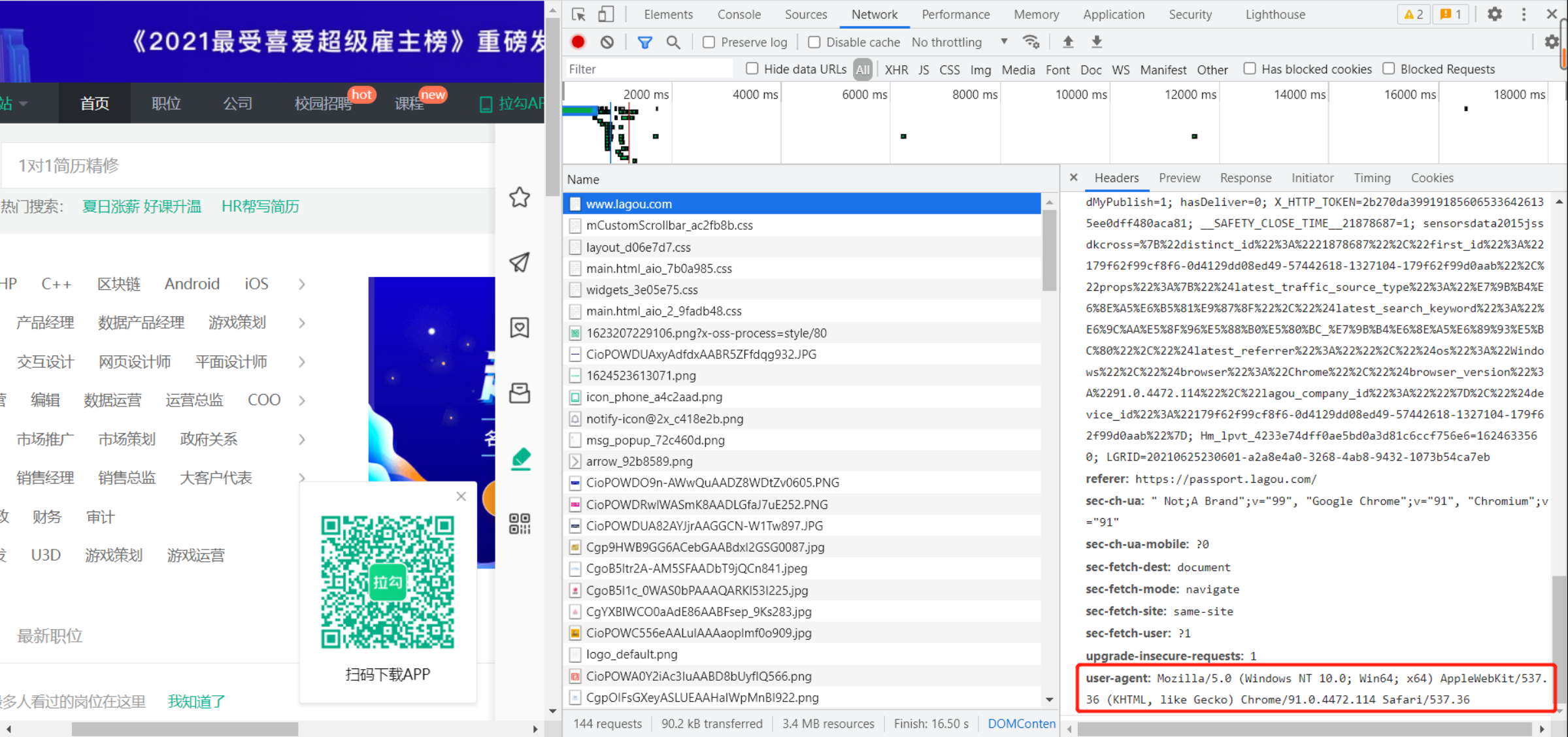
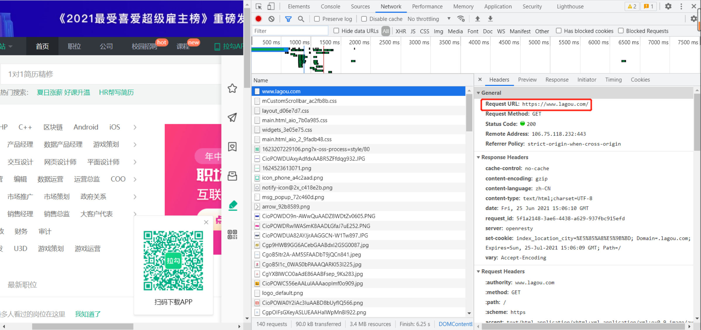
 2，Htmls页面解析

 

 

 

 

 

 

 四，程序设计

1，数据爬取与采集

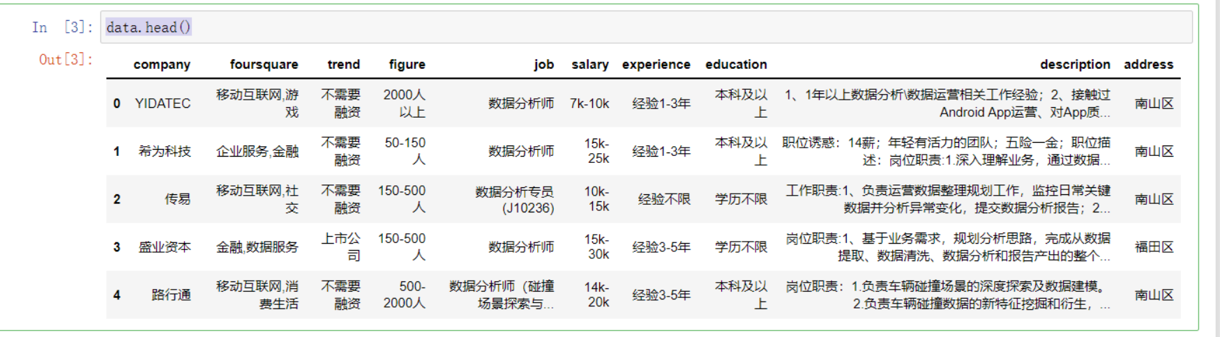
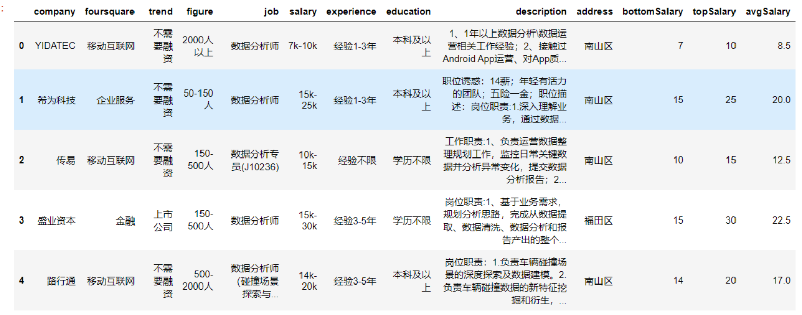
import numpy as npimport pandas as pdimport seaborn as snsimport jiebaimport jieba.analyseimport refrom wordcloud import WordCloudfrom matplotlib import pyplot as pltfrom matplotlib import style

style.use('ggplot')# from matplotlib.font_manager import FontPropertiesimport pprint# 让图表直接在jupyter中展示出来

%matplotlib inline# 解决中文乱码问题

plt.rcParams["font.sans-serif"] = 'SimHei'# 解决负号无法正常显示问题

plt.rcParams['axes.unicode_minus'] = False# import matplotlib as mpl

# 关闭警告信息import warnings

warnings.filterwarnings('ignore')

 

data = pd.read_csv('./lagou_DT.csv')

 

data.head()

 

 

 

 

 

data.info()

 

 

 

 

 

 

 

 

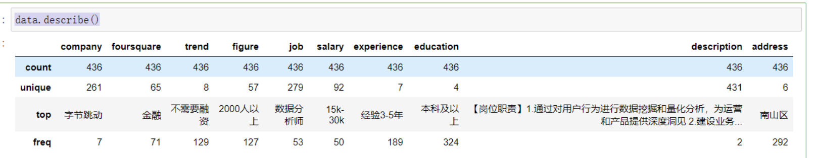
data.describe()

 

 

 

 

 

 

 

 2，对数据进行清洗和处理

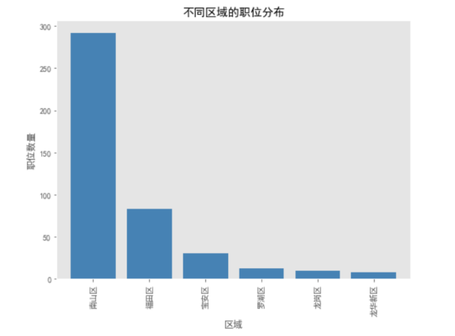
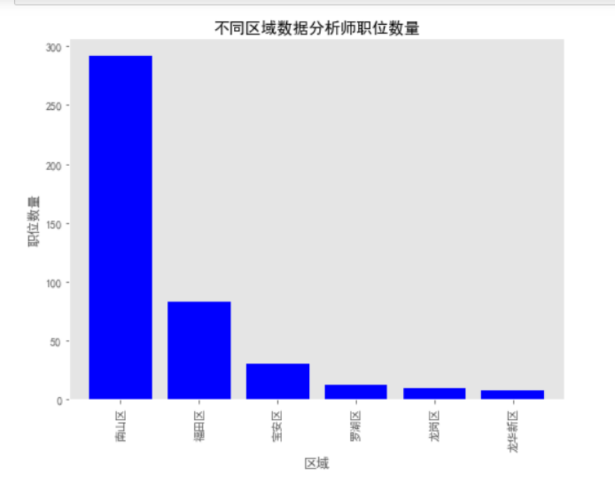
不同区域数据分析师职位的需求情况

1 plt.figure(figsize = (8,6))2 data['address'].value_counts().sort_values(ascending=False).plot.bar(width = 0.8,color = 'steelblue')3 plt.ylabel('职位数量')4 plt.xlabel('区域')5 plt.title('不同区域的职位分布')6 plt.grid(False)

 

 

 

 

 

 

 

 

plt.figure(figsize = (8,6))

data['address'].value_counts().sort_values(ascending = False).plot.bar(width = 0.8,color = 'blue')

plt.xlabel('区域')

plt.ylabel('职位数量')

plt.title('不同区域数据分析师职位数量')

plt.grid(False)

 

 

 

 

 

 

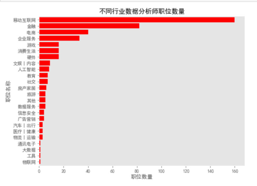
不同行业数据分析师岗位的需求情况

# 存在多个行业，只取第一个

clean_foursquare = [str(i.split(',')[0]) for i in data.foursquare]

data['foursquare'] = clean_foursquare

 

plt.figure(figsize = (8,6))

data['foursquare'].value_counts().sort_values(ascending = True).plot.barh(width = 0.8,color = 'red')

plt.xlabel('职位数量')

plt.ylabel('职位名称')

plt.title('不同行业数据分析师职位数量')

plt.grid(False)

 

 

 

 

 

 

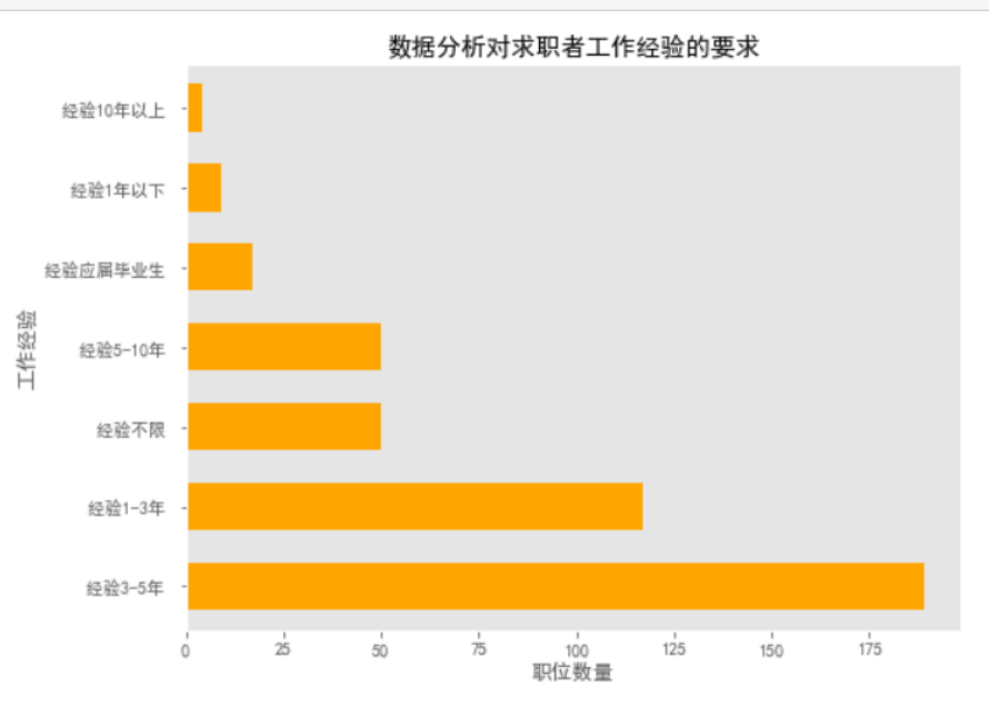
数据分析师对应聘者工作年限的要求

 

plt.figure(figsize = (8,6))

data['experience'].value_counts().plot.barh(width = 0.6,color = 'orange')

plt.xlabel('职位数量')

plt.ylabel('工作经验')

plt.title('数据分析对求职者工作经验的要求',loc = "center")

plt.grid(False)

 

 

 

 

 

 

 

数据分析师对应聘者工作年限的要求

plt.figure(figsize = (8,6))

data['experience'].value_counts().plot.barh(width = 0.6,color = 'orange')

plt.xlabel('职位数量')

plt.ylabel('工作经验')

plt.title('数据分析对求职者工作经验的要求',loc = "center")

plt.grid(False)

 

 

 

 

 

 

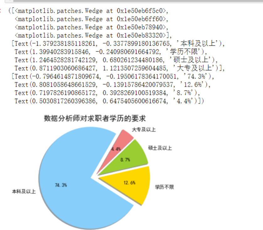
数据分析师对求职者学历的要求

education_count = data['education'].value_counts()

labels='本科及以上','学历不限','硕士及以上','大专及以上'

colors=[ 'lightskyblue', 'gold','yellowgreen', 'lightcoral']

explode=(0.1,0.1,0.1,0.1)

plt.axis('equal')

plt.title('数据分析师对求职者学历的要求',size = 15)

plt.pie(education_count,explode=explode,labels=labels,colors=colors,autopct='%1.1f%%',

        shadow=True,labeldistance=1.1,startangle=60,radius=1.2)

 

 

 

 

 

数据分析师的薪酬范围分布

# 去除字段中'k'或'K'字符

clean_salary = [re.sub('[k|K]','',i) for i in data.salary]

# 将salary数据转换为DataFrame格式

salary = pd.DataFrame(clean_salary,columns = ['salary'])

salary_s = pd.DataFrame((x.split('-') for x in salary['salary']),columns = ['bottomSalary','topSalary'])# 更改字段格式

salary_s['bottomSalary']=salary_s['bottomSalary'].astype(np.int)

salary_s['topSalary']=salary_s['topSalary'].astype(np.int)

# 计算平均值

salary_avg = [(salary_s['bottomSalary'][i] + salary_s['topSalary'][i])/2 for i in range(len(salary_s))]

salary_s['avgSalary'] = salary_avg# for i in range(len(salary_s)):

#     avg.append((salary_s['bottomSalary'][i]+salary_s['topSalary'][i])/2)

# salary_s['avgSalary']=avg

# 将salary_s表与原表进行拼接

data = pd.merge(data,salary_s,right_index=True,left_index=True)

data.head()

 

 

 

 

 

plt.figure(figsize = (8,6))

plt.hist(data['avgSalary'],bins=16,color='green')

plt.axis('tight')

plt.title('薪酬分布')

plt.xlabel('每月薪酬（单位：K/月）')

plt.ylabel('职位数量')

plt.grid(False)

 

 

 

 

 

 

公司规模与薪酬之间的关系

data['figure'] = data['figure'].map(str.strip)

data.groupby(['figure']).count()

 

size1=data.loc[data['figure'] == '15-50人',['figure','avgSalary']]

size2=data.loc[data['figure'] == '50-150人',['figure','avgSalary']]

size3=data.loc[data['figure'] == '150-500人',['figure','avgSalary']]

size4=data.loc[data['figure'] == '500-2000人',['figure','avgSalary']]

size5=data.loc[data['figure'] == '2000人以上',['figure','avgSalary']]

 

plt.figure(figsize = (20,8))

plt.xlabel('公司规模')

plt.ylabel('平均薪酬（K/月）')

plt.title('公司规模与平均薪酬')

plt.grid(False)

plt.boxplot((size1['avgSalary'],size2['avgSalary'],size3['avgSalary'],size4['avgSalary'],size5['avgSalary']),

            labels=('15-50人','50-150人','150-500人','500-2000人','2000人以上'))# plt.grid(color='#95a5a6',linestyle='--',linewidth=0.8,axis='y',alpha=0.4)

 

 

 

 

 

 

 

 

 

 

 

 

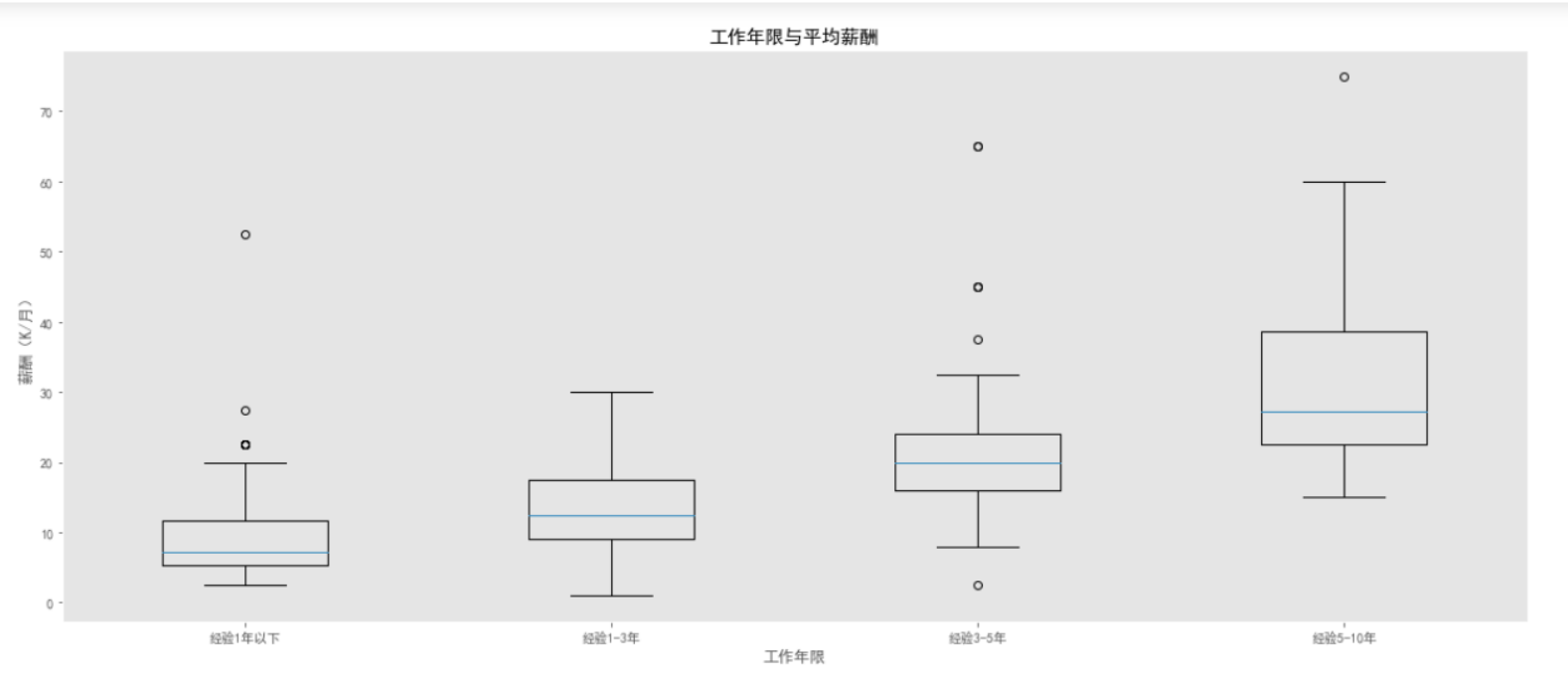
工作经验与薪酬的关系

data['experience'] = data['experience'].map(str.strip)

# 把经验应届毕业生和经验不限归为经验1年以下for i in range(len(data['experience'])):

    if data['experience'][i] in ['经验应届毕业生','经验不限']:

        data['experience'][i]='经验1年以下'# data['experience']

year1=data.loc[data['experience'] == '经验1年以下',['experience','avgSalary']]

year2=data.loc[data['experience'] == '经验1-3年',['experience','avgSalary']]

year3=data.loc[data['experience'] == '经验3-5年',['experience','avgSalary']]

year4=data.loc[data['experience'] == '经验5-10年',['experience','avgSalary']]

 

plt.figure(figsize = (20,8))

plt.xlabel('工作年限')

plt.ylabel('薪酬（K/月）')

plt.title('工作年限与平均薪酬')

plt.grid(False)# plt.grid(color='#95a5a6',linestyle='--',linewidth=0.8,axis='y',alpha=0.4)

plt.boxplot((year1['avgSalary'],year2['avgSalary'],year3['avgSalary'],year4['avgSalary']),

            labels=('经验1年以下','经验1-3年','经验3-5年','经验5-10年'))

 

 

 

 

 

 

 

 

 

 

 

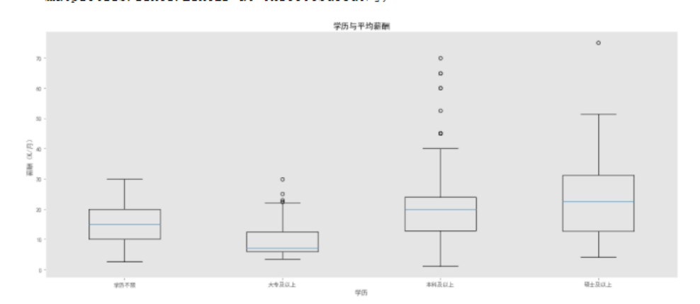
学历对薪酬的影响

data['education']=data['education'].map(str.strip)

 

edu1=data.loc[data['education'] == '学历不限',['education','avgSalary']]

edu2=data.loc[data['education'] == '大专及以上',['education','avgSalary']]

edu3=data.loc[data['education'] == '本科及以上',['education','avgSalary']]

edu4=data.loc[data['education'] == '硕士及以上',['education','avgSalary']]

 

plt.figure(figsize = (20,8))

plt.xlabel('学历')

plt.ylabel('薪酬（K/月）')

plt.title('学历与平均薪酬')

plt.grid(False)# plt.grid(color='#95a5a6',linestyle='--',linewidth=0.8,axis='y',alpha=0.4)

plt.boxplot((edu1['avgSalary'],edu2['avgSalary'],edu3['avgSalary'],edu4['avgSalary']),labels=('学历不限','大专及以上','本科及以上','硕士及以上'))

 

 

 

 

 

 

 

 

 

 

 职业技能关键词

 

# 把每个岗位描述连接起来保存在文件中

description_text = ' '.join([i for i in data['description']])

 

with open('des.txt','w',encoding = 'utf-8') as f:

    f.write(description_text)

    f.close()

 

text = open('des.txt', 'r',encoding='utf-8').read()

stop_word = ['岗位职责','任职要求','工作职责','岗位要求','任职资格','本科及以上学历','本科以上学历','职位描述',

             '工作职责','岗位职责1','职位诱惑','职位要求','任职要求1','工作职责1','职位职责','计算机','数据分析',

             'and','to','with','the','in','for','of']

wordcloud = WordCloud(font_path="./SimHei.ttf",

                      stopwords=stop_word,  # 去掉停用词

                      max_words=100,

                      width=2000,

                      height=1200).generate(text)# 保存词云

wordcloud.to_file('DT.jpg')# 显示词云文件plt.imshow(wordcloud)

plt.axis("off")

plt.show()

 

 

 

 

 

完整代码：

  

1，数据爬取与采集

import numpy as npimport pandas as pdimport seaborn as snsimport jiebaimport jieba.analyseimport refrom wordcloud import WordCloudfrom matplotlib import pyplot as pltfrom matplotlib import style

style.use('ggplot')# from matplotlib.font_manager import FontPropertiesimport pprint# 让图表直接在jupyter中展示出来

%matplotlib inline# 解决中文乱码问题

plt.rcParams["font.sans-serif"] = 'SimHei'# 解决负号无法正常显示问题

plt.rcParams['axes.unicode_minus'] = False# import matplotlib as mpl

# 关闭警告信息import warnings

warnings.filterwarnings('ignore')

 

data = pd.read_csv('./lagou_DT.csv')

 

data.head()


 

 

 

 

 

 

 

 

 

 

 

 

 

 

data.info()

 

 

 

 

data.describe()

 

 

 

 2，对数据进行清洗和处理

不同区域数据分析师职位的需求情况
1 plt.figure(figsize = (8,6))2 data['address'].value_counts().sort_values(ascending=False).plot.bar(width = 0.8,color = 'steelblue')3 plt.ylabel('职位数量')4 plt.xlabel('区域')5 plt.title('不同区域的职位分布')6 plt.grid(False)

 

 

 

 

 

plt.figure(figsize = (8,6))

data['address'].value_counts().sort_values(ascending = False).plot.bar(width = 0.8,color = 'blue')

plt.xlabel('区域')

plt.ylabel('职位数量')

plt.title('不同区域数据分析师职位数量')

plt.grid(False)

 

 

 

 

不同行业数据分析师岗位的需求情况
# 存在多个行业，只取第一个

clean_foursquare = [str(i.split(',')[0]) for i in data.foursquare]

data['foursquare'] = clean_foursquare

 

plt.figure(figsize = (8,6))

data['foursquare'].value_counts().sort_values(ascending = True).plot.barh(width = 0.8,color = 'red')

plt.xlabel('职位数量')

plt.ylabel('职位名称')

plt.title('不同行业数据分析师职位数量')

plt.grid(False)

 

 

 

数据分析师对应聘者工作年限的要求
 

plt.figure(figsize = (8,6))

data['experience'].value_counts().plot.barh(width = 0.6,color = 'orange')

plt.xlabel('职位数量')

plt.ylabel('工作经验')

plt.title('数据分析对求职者工作经验的要求',loc = "center")

plt.grid(False)

 

 

 

 

数据分析师对应聘者工作年限的要求
plt.figure(figsize = (8,6))

data['experience'].value_counts().plot.barh(width = 0.6,color = 'orange')

plt.xlabel('职位数量')

plt.ylabel('工作经验')

plt.title('数据分析对求职者工作经验的要求',loc = "center")

plt.grid(False)

 

 

 





数据分析师对求职者学历的要求
education_count = data['education'].value_counts()

labels='本科及以上','学历不限','硕士及以上','大专及以上'

colors=[ 'lightskyblue', 'gold','yellowgreen', 'lightcoral']

explode=(0.1,0.1,0.1,0.1)

plt.axis('equal')

plt.title('数据分析师对求职者学历的要求',size = 15)

plt.pie(education_count,explode=explode,labels=labels,colors=colors,autopct='%1.1f%%',

        shadow=True,labeldistance=1.1,startangle=60,radius=1.2)

 

 





 

数据分析师的薪酬范围分布
# 去除字段中'k'或'K'字符

clean_salary = [re.sub('[k|K]','',i) for i in data.salary]

# 将salary数据转换为DataFrame格式

salary = pd.DataFrame(clean_salary,columns = ['salary'])

salary_s = pd.DataFrame((x.split('-') for x in salary['salary']),columns = ['bottomSalary','topSalary'])# 更改字段格式

salary_s['bottomSalary']=salary_s['bottomSalary'].astype(np.int)

salary_s['topSalary']=salary_s['topSalary'].astype(np.int)

# 计算平均值

salary_avg = [(salary_s['bottomSalary'][i] + salary_s['topSalary'][i])/2 for i in range(len(salary_s))]

salary_s['avgSalary'] = salary_avg# for i in range(len(salary_s)):

#     avg.append((salary_s['bottomSalary'][i]+salary_s['topSalary'][i])/2)

# salary_s['avgSalary']=avg

# 将salary_s表与原表进行拼接

data = pd.merge(data,salary_s,right_index=True,left_index=True)

data.head()

 

 






 

plt.figure(figsize = (8,6))

plt.hist(data['avgSalary'],bins=16,color='green')

plt.axis('tight')

plt.title('薪酬分布')

plt.xlabel('每月薪酬（单位：K/月）')

plt.ylabel('职位数量')

plt.grid(False)

 

 




 

公司规模与薪酬之间的关系
data['figure'] = data['figure'].map(str.strip)

data.groupby(['figure']).count()

 






size1=data.loc[data['figure'] == '15-50人',['figure','avgSalary']]

size2=data.loc[data['figure'] == '50-150人',['figure','avgSalary']]

size3=data.loc[data['figure'] == '150-500人',['figure','avgSalary']]

size4=data.loc[data['figure'] == '500-2000人',['figure','avgSalary']]

size5=data.loc[data['figure'] == '2000人以上',['figure','avgSalary']]

 

plt.figure(



figsize = (20,8))

plt.xlabel('公司规模')

plt.ylabel('平均薪酬（K/月）')

plt.title('公司规模与平均薪酬')

plt.grid(False)

plt.boxplot((size1['avgSalary'],size2['avgSalary'],size3['avgSalary'],size4['avgSalary'],size5['avgSalary']),

            labels=('15-50人','50-150人','150-500人','500-2000人','2000人以上'))# plt.grid(color='#95a5a6',linestyle='--',linewidth=0.8,axis='y',alpha=0.4)

 

 

 

 

 

 

 

工作经验与薪酬的关系
data['experience'] = data['experience'].map(str.strip)

# 把经验应届毕业生和经验不限归为经验1年以下for i in range(len(data['experience'])):

    if data['experience'][i] in ['经验应届毕业生','经验不限']:

        data['experience'][i]='经验1年以下'# data['experience']

year1=data.loc[data['experience'] == '经验1年以下',['experience','avgSalary']]

year2=data.loc[data['experience'] == '经验1-3年',['experience','avgSalary']]

year3=data.loc[data['experience'] == '经验3-5年',['experience','avgSalary']]

year4=data.loc[data['experience'] == '经验5-10年',['experience','avgSalary']]

 





plt.figure(figsize = (20,8))

plt.xlabel('工作年限')

plt.ylabel('薪酬（K/月）')

plt.title('工作年限与平均薪酬')

plt.grid(False)# plt.grid(color='#95a5a6',linestyle='--',linewidth=0.8,axis='y',alpha=0.4)

plt.boxplot((year1['avgSalary'],year2['avgSalary'],year3['avgSalary'],year4['avgSalary']),

            labels=('经验1年以下','经验1-3年','经验3-5年','经验5-10年'))

 

 

 

 

 

 

学历对薪酬的影响
data['education']=data['education'].map(str.strip)

 

edu1=data.loc[data['education'] == '学历不限',['education','avgSalary']]

edu2=data.loc[data['education'] == '大专及以上',['education','avgSalary']]

edu3=data.loc[data['education'] == '本科及以上',['education','avgSalary']]

edu4=data.loc[data['education'] == '硕士及以上',['education','avgSalary']]

 






plt.figure(figsize = (20,8))

plt.xlabel('学历')

plt.ylabel('薪酬（K/月）')

plt.title('学历与平均薪酬')

plt.grid(False)# plt.grid(color='#95a5a6',linestyle='--',linewidth=0.8,axis='y',alpha=0.4)

plt.boxplot((edu1['avgSalary'],edu2['avgSalary'],edu3['avgSalary'],edu4['avgSalary']),labels=('学历不限','大专及以上','本科及以上','硕士及以上'))


 

 

 

 

 

 

 职业技能关键词
 

# 把每个岗位描述连接起来保存在文件中

description_text = ' '.join([i for i in data['description']])

 

with open('des.txt','w',encoding = 'utf-8') as f:

    f.write(description_text)

    f.close()

 

text = open('des.txt', 'r',encoding='utf-8').read()

stop_word = ['岗位职责','任职要求','工作职责','岗位要求','任职资格','本科及以上学历','本科以上学历','职位描述',

             '工作职责','岗位职责1','职位诱惑','职位要求','任职要求1','工作职责1','职位职责','计算机','数据分析',

             'and','to','with','the','in','for','of']

wordcloud = WordCloud(font_path="./SimHei.ttf",

                      stopwords=stop_word,  # 去掉停用词

                      max_words=100,

                      width=2000,

                      height=1200).generate(text)# 保存词云

wordcloud.to_file('DT.jpg')# 显示词云文件plt.imshow(wordcloud)

plt.axis("off")

plt.show()

 

 

 五，总结

通过上面的分析，可以得到如下结论：

1，在深圳数据分析师岗位需求主要集中在南山、福田，即互联网聚集地，总体待遇较高（基本上在8K以上），学历要求不是特别高（本科以上），大厂需求量较大，大量的工作经验需求集中在1-3年。

2，数据分析师分布的行业领域主要是移动互联网行业，不过也开始向传统行业（例如金融、教育）渗透。

3，数据分析师技能具备的频率排在前列的有：SQL，Python，数学统计，对数据敏感，Excel， SAS，SPSS, Hadoop，机器学习等，其中数学统计、SQL、Python、Excel是必备技能。

4，机器学习、大数据挖掘是走向高薪的正确方向。

 

在整个设计的过程中，我学到了很多新知识，增长了见识。我想这是一次意志的磨练，是对我实际能力的一次提升，也会对我未来的学习和工作有很大的帮助。需要改进的建议在于该网络爬虫程序只获取了单个网站的就业信息，下一步的重点应该放在如何进行多数据源的就业信息获取，以获得更加全面的就业信息。