行分控模型的建立

数据预处理：

# -*- coding: utf-8 -*-
"""
Created on Tue Mar 29 18:52:22 2022

@author: 86150
"""

#-*- coding: utf-8 -*-
def cm_plot(y, yp):
   
  from sklearn.metrics import confusion_matrix #导入混淆矩阵函数
 
  cm = confusion_matrix(y, yp) #混淆矩阵
   
  import matplotlib.pyplot as plt #导入作图库
  plt.matshow(cm, cmap=plt.cm.Greens) #画混淆矩阵图，配色风格使用cm.Greens，更多风格请参考官网。
  plt.colorbar() #颜色标签
   
  for x in range(len(cm)): #数据标签
    for y in range(len(cm)):
      plt.annotate(cm[x,y], xy=(x, y), horizontalalignment='center', verticalalignment='center')
   
  plt.ylabel('True label') #坐标轴标签
  plt.xlabel('Predicted label') #坐标轴标签
  return plt

# -*- coding: utf-8 -*-
"""
Created on Tue Mar 29 18:52:22 2022

@author: 86150
"""

#-*- coding: utf-8 -*-
def cm_plot(y, yp):
   
  from sklearn.metrics import confusion_matrix #导入混淆矩阵函数
 
  cm = confusion_matrix(y, yp) #混淆矩阵
   
  import matplotlib.pyplot as plt #导入作图库
  plt.matshow(cm, cmap=plt.cm.Greens) #画混淆矩阵图，配色风格使用cm.Greens，更多风格请参考官网。
  plt.colorbar() #颜色标签
   
  for x in range(len(cm)): #数据标签
    for y in range(len(cm)):
      plt.annotate(cm[x,y], xy=(x, y), horizontalalignment='center', verticalalignment='center')
   
  plt.ylabel('True label') #坐标轴标签
  plt.xlabel('Predicted label') #坐标轴标签
  return plt

 

 

二、神经网络算法建立模型

 

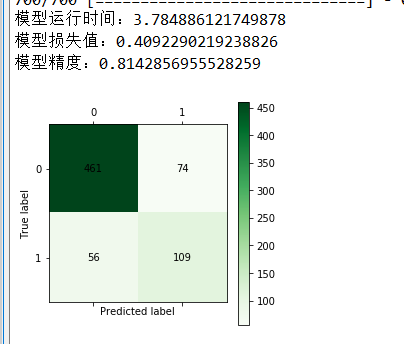
# -*- coding: utf-8 -*-
"""
Created on Tue Mar 29 18:55:21 2022

@author: 86150
"""

import pandas as pd
import numpy as np
#导入划分数据集函数
from sklearn.linear_model import LogisticRegression as LR
from sklearn.model_selection import train_test_split
#读取数据
datafile = 'data5/bankloan.xls'#文件路径
data = pd.read_excel(datafile)
x = data.iloc[:,:8]
y = data.iloc[:,8]
#划分数据集
x_train, x_test, y_train, y_test = train_test_split(x, y, test_size=0.2, random_state=100)
#导入模型和函数
from tensorflow.keras.models import Sequential
from tensorflow.keras.layers import Dense,Dropout
#导入指标
from tensorflow.keras.metrics import BinaryAccuracy
#导入时间库计时
import time
start_time = time.time()
#-------------------------------------------------------#
model = Sequential()
model.add(Dense(input_dim=8,units=800,activation='relu'))#激活函数relu
model.add(Dropout(0.5))#防止过拟合的掉落函数
model.add(Dense(input_dim=800,units=400,activation='relu'))
model.add(Dropout(0.5))
model.add(Dense(input_dim=400,units=1,activation='sigmoid'))
 
model.compile(loss='binary_crossentropy', optimizer='adam',metrics=[BinaryAccuracy()])
model.fit(x_train,y_train,epochs=100,batch_size=128)    #调参 epochs:训练次数，此处为100次
loss,binary_accuracy = model.evaluate(x,y,batch_size=128)
#--------------------------------------------------------#
end_time = time.time()
run_time = end_time-start_time#运行时间
 
print('模型运行时间：{}'.format(run_time))
print('模型损失值：{}'.format(loss))
print('模型精度：{}'.format(binary_accuracy))
 
yp = model.predict(x).reshape(len(y))
yp = np.around(yp,0).astype(int) #转换为整型
from cm_plot import *  # 导入自行编写的混淆矩阵可视化函数
 
cm_plot(y,yp).show()  # 显示混淆矩阵可视化结果

 

 

三、SVM支持向量机算法模型

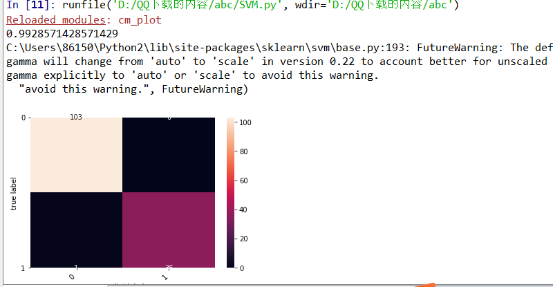
# -*- coding: utf-8 -*-
"""
Created on Tue Mar 29 19:08:49 2022

@author: 86150
"""

from sklearn import svm
from sklearn.metrics import accuracy_score
from sklearn.metrics import confusion_matrix
from matplotlib import pyplot as plt
import seaborn as sns
import pandas as pd
import numpy as np
from sklearn.model_selection import train_test_split
data_load = "data5/bankloan.xls"
data = pd.read_excel(data_load)
data.describe()
data.columns
data.index
## 转为np 数据切割
X = np.array(data.iloc[:,0:-1])
y = np.array(data.iloc[:,-1])
X_train, X_test, y_train, y_test = train_test_split(X, y, random_state=1, train_size=0.8, test_size=0.2, shuffle=True)
svm = svm.SVC()
svm.fit(X_test,y_test)
y_pred = svm.predict(X_test)
accuracy_score(y_test, y_pred)
print(accuracy_score(y_test, y_pred))
cm = confusion_matrix(y_test, y_pred)
heatmap = sns.heatmap(cm, annot=True, fmt='d')
heatmap.yaxis.set_ticklabels(heatmap.yaxis.get_ticklabels(), rotation=0, ha='right')
heatmap.xaxis.set_ticklabels(heatmap.xaxis.get_ticklabels(), rotation=45, ha='right')
plt.ylabel("true label")
plt.xlabel("predict label")
plt.show()