XGBoost 原生版本和sklearn接口版本的使用（泰坦尼克数据）

2021.3.11补充：

官网地址：https://xgboost.readthedocs.io/en/latest/python/python_api.html

DMatrix

是XGBoost中使用的数据矩阵。DMatrix是XGBoost使用的内部数据结构，它针对内存效率和训练速度进行了优化

class xgboost.DMatrix(data, label=None, *, weight=None, base_margin=None, missing=None, silent=False, feature_names=None, 
feature_types=None, nthread=None, group=None, qid=None, label_lower_bound=None, label_upper_bound=None, feature_weights=None, enable_categorical=False)

参数：

data：即是入模特征的表，可以是多种数据类型，df，或者numpy.array 等等

label：即是y值，数据类型同上

还有一些我们暂时不需要，平时使用到的一般都是这两个变量，下面说一下属性

get_label()：可以得到y值

其余的需要到再阅读API文档

train

xgboost.train(params, dtrain, num_boost_round=10, evals=(), obj=None, feval=None, maximize=None, 
early_stopping_rounds=None, evals_result=None, verbose_eval=True, xgb_model=None, callbacks=None)

参数：

params：参数，是dict形式

dtrain（DMatrix）：要训练的数据，也就是上面xgboost.DMatrix后得到的数据

num_boost_round（int）：提升迭代的次数

evals（对列表（DMatrix，字符串））–在训练期间将评估其度量的验证集列表。验证指标将帮助我们跟踪模型的性能，也就是训练集和测试集（train-auc:0.92495 valid-auc:0.91495）展示成这个样子，平时有人会写成watchlist

obj（function）–自定义的目标函数

early_stopping_rounds（int）：如果迭代完还是找不到最优次数，那么就是使用这个值最为最优迭代次数

verbose_eval（布尔值或整数）：每隔n次迭代一次

返回就是一个模型，API没有详细的说明，但是我们知道有如下属性或者方法：

函数/方法：['attr', 'attributes', 'boost', 'copy', 'dump_model', 'eval', 'eval_set', 'get_dump', 'get_fscore', 'get_score', 'get_split_value_histogram', 'inplace_predict', 'load_config', 'load_model', 'load_rabit_checkpoint', 'predict', 'save_config', 'save_model', 'save_rabit_checkpoint', 'save_raw', 'set_attr', 'set_param', 'trees_to_dataframe', 'update']

属性：['best_iteration', 'best_ntree_limit', 'best_score', 'booster', 'feature_names', 'feature_types', 'handle']

`xgboost.cv`

xgboost.cv(params, dtrain, num_boost_round=10, nfold=3, stratified=False, folds=None, metrics=(), obj=None, feval=None, maximize=None, 
early_stopping_rounds=None, fpreproc=None, as_pandas=True, verbose_eval=None, show_stdv=True, seed=0, callbacks=None, shuffle=True)

主要用来寻找最优参数的，通过交叉验证去寻找最优参数

params（dict）–助推器参数。
dtrain（DMatrix）–要训练的数据。
num_boost_round（int）–提升迭代的次数。通常表达成num_boost_round=model.get_params()['n_estimators']
nfold（int）– CV的折叠数。
stratified（布尔）–执行分层采样。不常用，需要分层采样时再使用
folds（KFold或StratifiedKFold实例或折叠索引列表）– Sklearn KFolds或StratifiedKFolds对象。或者，可以显式传递每个折叠的样本索引。对于n折叠，折叠应n为元组的长度列表。每个元组在(in,out)哪里in是用作n第三折的训练样本out的索引列表，并且是用作n第三折的测试样本的索引列表。
metrics（字符串或字符串列表）–在CV中要观察的评估指标。
obj（function）–自定义目标函数。
feval（函数）–自定义评估函数。
maximize（布尔）–是否最大化盛宴。
early_stopping_rounds（int）–激活提前停止。交叉验证度量标准（通过CV折叠计算得出的验证度量标准的平均值）需要在每个Early_stopping_rounds回合中至少改善一次，以继续进行训练。评估历史记录中的最后一个条目将代表最佳迭代。如果在params中给定的eval_metric参数中有多个度量标准，则最后一个度量标准将用于提前停止。
fpreproc（函数）–预处理函数，它接受（dtrain，dtest，param）并返回这些函数的转换版本。
as_pandas（bool，默认为True）–安装pandas时返回pd.DataFrame。如果未安装False或pandas，则返回np.ndarray
verbose_eval（bool，int或None，默认为None）–是否显示进度。如果为None，则返回np.ndarray时将显示进度。如果为True，则进度将在提升阶段显示。如果给定一个整数，则将在每个给定的verbose_eval提升阶段显示进度。
show_stdv（bool，默认为True）–是否显示进行中的标准偏差。结果不受影响，并且始终包含std。
seed（int）–用于生成折叠的种子（传递给numpy.random.seed）
callbacks (list of callback functions) –在每次迭代结束时应用的回调函数列表。通过使用Callback API可以使用预定义的回调。例子：
```
[xgb.callback.LearningRateScheduler(custom_rates)]
```

一般这样使用

def model_cv(model, X, y, cv_folds=5, early_stopping_rounds=50, seed=0):
    xgb_param = model.get_xgb_params()
    xgtrain = xgb.DMatrix(X, label=y)
    cvresult = xgb.cv(xgb_param, xgtrain, num_boost_round=model.get_params()['n_estimators'], nfold=cv_folds,
                    metrics='auc', seed=seed, callbacks=[
            xgb.callback.print_evaluation(show_stdv=False),
            xgb.callback.early_stop(early_stopping_rounds)
       ])
    num_round_best = cvresult.shape[0] - 1
    print('Best round num: ', num_round_best)
    return num_round_best


num_round = 500
seed = 0
max_depth = 4
min_child_weight = 1000
gamma = 0
subsample = 0.8
colsample_bytree = 0.8
scale_pos_weight = 1
reg_alpha = 1
reg_lambda = 1e-5
learning_rate = 0.1
model = XGBClassifier(learning_rate=learning_rate, n_estimators=num_round, max_depth=max_depth,
                      min_child_weight=min_child_weight, gamma=gamma, subsample=subsample, reg_alpha=reg_alpha,
                      reg_lambda=reg_lambda, colsample_bytree=colsample_bytree, objective='binary:logistic',
                      nthread=4, scale_pos_weight=scale_pos_weight, seed=seed)
num_round = model_cv(model,X , y)

2. 两个版本的区别

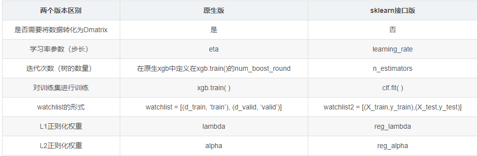
建议还是使用原生版本

一、XGBoost的原生版本参数介绍

1.1 General Parameters通用参数

booster [default=gbtree]：可选项为gbtree，gblinear或dart；其中gbtree和dart是使用基于树模型的，而gblinear是使用基于线性模型的；
silent [default=0]：0表示输出运行信息，1表示不输出；
nthread [如果不进行设置，默认是最大线程数量]：表示XGBoost运行时的并行线程数量；
disable_default_eval_metric [default=0]：标记以禁用默认度量标准。设置 >0 表示禁用；
num_pbuffer [通过XGBoost自动设置，不需要用户来设置]：预测缓冲区的大小，通常设置为训练实例的数量；
num_feature [通过XGBoost自动设置，不需要用户来设置]：被使用在boosting中的特征维度，设置为最大化的特征维度

1.2 Parameters for Tree Booster：

eta (default=0.3, 别名: learning_rate) ：eta表示学习率：range：[0, 1] ，作用：防止过拟合；
gamma [default=0, 别名: min_split_loss]：在树的叶节点上进一步分区所需的最小化损失减少，gamma越大算法越保守 range:[0, ∞]；
max_depth [default=6]：表示树的深度，值越大模型越复杂，越容易过拟合。0表示不限制；
min_child_weight [default=1]：子节点所需要的最小样本权重之和。如果一个叶子节点的样本权重和小于min_child_weight结束节点进一步的切分。在线性回归模型中，这个参数是指建立每个模型所需要的最小样本数。该值越大，算法越保守；
max_delta_step [default=0]：我们允许每个叶子输出的最大的delta step，该值为0，表示不限制。该值为正数，可以帮助使更新步骤更加保守。通常该参数不需要设置，但是在logistic回归中，分类类别极度不平衡的时候，将该值设置在1_10之间可以帮助控制更新步骤；
subsample [default=1]：训练数据的子样本，subsample=n，表示在训练数据中随机采样n%的样本，可以防止过拟合。 range：(0, 1] ；
lambda [default=1, 别名: reg_lambda]： L2正则化项系数；
alpha [default=0, 别名: reg_alpha]： L1正则化项系数；
tree_method string [default= auto]：在分布式和外存的版本中，仅支持 tree_method=approx；可选项为：auto, exact, approx, hist, gpu_exact, gpu_hist
- auto：表示使用启发式的方法来选择使运行速度最快的算法，如下：
  - 对于小到中等的数据集，Exact Greedy Algorithm将被使用；
  - 对于大数据集，Approximate Algorithm将被使用；
  - 因为以前的行为总是在单个机器中使用Exact Greedy Algorithm，所以当选择Approximate Algorithm来通知该选择时，用户将得到消息。
- exact：Exact Greedy Algorithm
- approx：Approximate Algorithm
- hist：快速直方图优化近似贪心算法。它使用了一些可以改善性能的方法，例如bins caching；
- gpu_exact：在GPU上执行Exact Greedy Algorithm；
- gpu_hist：在GPU上执行hist算法；
max_leaves [default=0]：设置叶节点的最大数量，仅仅和当row_policy=lossguide才需要被设置；
max_bin, [default=256]：仅仅tree_method=hist时，该方法需要去设置。bucket连续特征的最大离散bins数量；

1.3 学习任务参数（Learning Task Parameters）

objective [default=reg:linear]
- reg:linear：线性回归；
- reg:logistic：逻辑回归；
- binary:logistic：二分类逻辑回归，输出概率，难怪后面会有>0.5的操作；
- binary:logitraw：二分类逻辑回归，在logistic transformation之前输出score；
- binary:hinge：二分类的hinge损失，让预测为0或1，而不是概率；
- multi:softmax：多分类的使用softmax目标函数，使用此含参数时需要指定多分类分为几类，设置num_class=n；
- multi:softprob: 和softmax相同，但是输出的是每个样本点属于哪个类的预测概率值；
- rank:pairwise：使用XGBoost做排序任务使用的。
base_score [default=0.5]：所有实例的初始预测分数，全局偏差。对于有足够的迭代数目，改变该值将不会太多的影响；
eval_metric [default according to objective] ：默认：根据objective参数(回归：rmse, 分类：error)。还有许多可以自己查官方API。

二、XGBoost的sklearn接口版本参数介绍

因为XGBoost是使用的是一堆CART树进行集成的，而CART(Classification And Regression Tree)树即可用作分类也可用作回归，这里仅仅介绍XGBoost的分类，回归问题类似，有需要请访问XGBoost API的官网进行查看。

class xgboost.XGBClassifier(max_depth=3, learning_rate=0.1, n_estimators=100, silent=True, objective='binary:logistic', booster='gbtree', n_jobs=1, nthread=None, gamma=0, min_child_weight=1, max_delta_step=0, subsample=1, colsample_bytree=1, colsample_bylevel=1, reg_alpha=0, reg_lambda=1, scale_pos_weight=1, base_score=0.5, random_state=0, seed=None, missing=None, **kwargs)

max_depth : int 表示基学习器的最大深度；
learning_rate : float 表示学习率，相当于原生版本的 "eta";
n_estimators: int 表示去拟合的boosted tree数量；
silent：boolean 表示是否在运行boosting期间打印信息；
objective：string or callable 指定学习任务和相应的学习目标或者一个自定义的函数被使用，具体看原生版本的objective；
booster：string 指定要使用的booster，可选项为：gbtree，gblinear 或 dart；
n_jobs：int 在运行XGBoost时并行的线程数量。
gamma：float 在树的叶节点上进行进一步分区所需的最小损失的减少值，即加入新节点进入的复杂度的代价；
min_child_weight ： int 在子节点中实例权重的最小的和；
max_delta_step ： int 我们允许的每棵树的权重估计最大的delta步骤；
subsample ：float 训练样本的子采样率；
colsample_bytree ：float 构造每个树时列的子采样率。
colsample_bylevel ：float 在每一层中的每次切分节点时的列采样率；
reg_alpha ：float 相当于原生版本的alpha，表示L1正则化项的权重系数；
reg_lambda： float 相当于原生版本的lambda，表示L2正则化项的权重系数；
scale_pos_weight：float 用来平衡正负权重；
base_score：所有实例的初始预测分数，全局偏差；
random_state：int 随机种子；
missing：float，optional 需要作为缺失值存在的数据中的值。如果为None，则默认为np.nan。

三、代码

数据字典

survival------表示乘客是否存活；0=No，1=Yes
pclass------表示票的等级；1=1st，2=2nd，3=3rd
sex------表示乘客性别；
Age------表示乘客年龄
sibsp------表示在船上的兄弟姐妹加上配偶的数量
parch------表示在船上的父母加上子女的数量
ticket------表示票的编号
fare------表示票价
cabin------表示船舱编号
embarked------表示乘客登录的港口；C = Cherbourg, Q = Queenstown, S = Southampton

数据的特征处理

导入模块

import pandas as pd
import numpy as np
import matplotlib.pyplot as plt
import seaborn as sns
import xgboost as xgb
from sklearn.model_selection import train_test_split
from sklearn import preprocessing 
from sklearn.model_selection import GridSearchCV
from sklearn.linear_model import LogisticRegression
from sklearn.ensemble import RandomForestClassifier
from sklearn.ensemble import GradientBoostingClassifier
from sklearn.preprocessing import LabelEncoder
 
import warnings
warnings.filterwarnings('ignore')

导入训练集和测试集

train =pd.read_csv("D:\\Users\\Downloads\\《泰坦尼克号数据分析项目数据》\\train.csv", index_col=0)
test = pd.read_csv("D:/Users/Downloads/《泰坦尼克号数据分析项目数据》/test.csv", index_col=0)
train.info()  # 打印训练数据的信息

<class 'pandas.core.frame.DataFrame'>
Int64Index: 891 entries, 1 to 891
Data columns (total 11 columns):
 #   Column    Non-Null Count  Dtype  
---  ------    --------------  -----  
 0   Survived  891 non-null    int64  
 1   Pclass    891 non-null    int64  
 2   Name      891 non-null    object 
 3   Sex       891 non-null    object 
 4   Age       714 non-null    float64
 5   SibSp     891 non-null    int64  
 6   Parch     891 non-null    int64  
 7   Ticket    891 non-null    object 
 8   Fare      891 non-null    float64
 9   Cabin     204 non-null    object 
 10  Embarked  889 non-null    object 
dtypes: float64(2), int64(4), object(5)
memory usage: 83.5+ KB

从输出信息中可以看出训练集一共有891个样本,11个特征，所有数据所占的内存大小为83.5K；所有的特征中有两个特征缺失情况较为严重,一个是Age,一个是Cabin;一个缺失不严重Embarked；数据一共有三种类型,float64(2), int64(5), object(5)。

接下来就是对数据的缺失值进行处理，这里采用的方法是对连续值用该列的平均值进行填充，非连续值用该列的众数进行填充，还可以使用机器学习的模型对缺失值进行预测，用预测的值来填充缺失值，该方法这里不做介绍

def handle_na(train, test):  # 将Cabin特征删除
    fare_mean = train['Fare'].mean()  # 测试集的fare特征有缺失值，用训练数据的均值填充
    test.loc[pd.isnull(test.Fare), 'Fare'] = fare_mean
 
    embarked_mode = train['Embarked'].mode()  # 用众数填充
    train.loc[pd.isnull(train.Embarked), 'Embarked'] = embarked_mode[0]
    
    train.loc[pd.isnull(train.Age), 'Age'] = train['Age'].mean()  # 用均值填充年龄
    test.loc[pd.isnull(test.Age), 'Age'] = train['Age'].mean()
    return train, test
 
new_train, new_test = handle_na(train, test)  # 填充缺失值

由于Embarked，Sex，Pclass特征是离散特征，所以对其进行one-hot/get_dummies编码

# 对Embarked和male特征进行one-hot/get_dummies编码
new_train = pd.get_dummies(new_train, columns=['Embarked', 'Sex', 'Pclass'])
new_test = pd.get_dummies(new_test, columns=['Embarked', 'Sex', 'Pclass'])

然后再去除掉PassengerId，Name，Ticket，Cabin, Survived列，这里不使用这些特征做预测

target = new_train['Survived'].values
# 删除PassengerId，Name，Ticket，Cabin, Survived列,  且全部换成了数组的形式
df_train = new_train.drop(['Name','Ticket','Cabin','Survived'], axis=1).values
df_test = new_test.drop(['Name','Ticket','Cabin'], axis=1).values

不管是特征还是label都已经换成了数组（array）形式，可能模型接收的数据形式就是这样

使用原生态版本

X_train,X_test,y_train,y_test = train_test_split(df_train,target,test_size = 0.3,random_state = 1)
 
data_train = xgb.DMatrix(X_train, y_train)  # 使用XGBoost的原生版本需要对数据进行转化
data_test = xgb.DMatrix(X_test, y_test)  #这个是使用原生态版本必须要做的事情
 
param = {'max_depth': 5, 'eta': 1, 'objective': 'binary:logistic'}
watchlist = [(data_test, 'test'), (data_train, 'train')]  #这个参数需要特别注意一下
n_round = 3
booster = xgb.train(param, data_train, num_boost_round=n_round, evals=watchlist)  #这里也是
 
# 计算错误率
y_predicted = booster.predict(data_test)   #注意这里使用的测试集
y = data_test.get_label()   #这个函数是xgb.DMatrix里面的，具体还得看看怎么使用
 
accuracy = sum(y == (y_predicted > 0.5))  #sum（布尔型）时，只计算True的值
#这个首先y_predicted > 0.5返回的是布尔型的数据，而y又是0或者1，那么y == (y_predicted > 0.5)，当y=1且(y_predicted > 0.5)=True时，或者
#当y=0且(y_predicted > 0.5)=False时，返回的才是True，其余的都是False
accuracy_rate = float(accuracy) / len(y_predicted)
print ('样本总数：{0}'.format(len(y_predicted)))
print ('正确数目：{0}'.format(accuracy) )
print ('正确率：{0:.3f}'.format((accuracy_rate)))

[0]	test-error:0.231343	train-error:0.126806
[1]	test-error:0.227612	train-error:0.117175
[2]	test-error:0.223881	train-error:0.104334
样本总数：268
正确数目：208
正确率：0.776

sklearn 接口版本的用法

XGBoost的sklearn的接口版本用法与sklearn中的模型的用法相同，这里简单的进行使用

X_train,X_test,y_train,y_test = train_test_split(df_train,target,test_size = 0.3,random_state = 1)
 
model = xgb.XGBClassifier(max_depth=3, n_estimators=200, learn_rate=0.01) #使用时主要区别在这里，其实接口形式的和其他的模型用法基本一样
model.fit(X_train, y_train)  
test_score = model.score(X_test, y_test)  #也是使用测试集
print('test_score: {0}'.format(test_score))

test_score: 0.7723880597014925

使用其他模型看看区别如何

# 应用模型进行预测
from sklearn.model_selection import ShuffleSplit  #使用ShuffleSplit方法，可以随机的把数据打乱，然后分为训练集和测试集。可以指定测试集占比
model_lr = LogisticRegression()   #逻辑回归
model_rf = RandomForestClassifier(n_estimators=200)  #随机深林
model_xgb = xgb.XGBClassifier(max_depth=5, n_estimators=200, learn_rate=0.01)  #sklearn接口版本
models = [model_lr, model_rf, model_xgb]
model_name = ['LogisticRegression', '随机森林', 'XGBoost']
 
cv = ShuffleSplit(n_splits=3, test_size=0.3, random_state=1)
for i in range(3):
    print(model_name[i] + ":")
    model = models[i]
    for train, test in cv.split(df_train):    
        model.fit(df_train[train], target[train])
        train_score = model.score(df_train[train], target[train])
        test_score = model.score(df_train[test], target[test])
        print('train score: {0:.5f} \t test score: {0:.5f}'.format(train_score, test_score))

LogisticRegression:
train score: 0.81220 	 test score: 0.81220
train score: 0.81701 	 test score: 0.81701
train score: 0.82183 	 test score: 0.82183
随机森林:
train score: 0.98876 	 test score: 0.98876
train score: 0.99037 	 test score: 0.99037
train score: 0.99037 	 test score: 0.99037
XGBoost:
train score: 0.95185 	 test score: 0.95185
train score: 0.96629 	 test score: 0.96629
train score: 0.95345 	 test score: 0.95345

备注一下：random_state真的是一个很神奇的参数，值不一样得到的结果也会有很大的区别，导致上面的结果差异这么大

下面我就做了一个循环，记录每次的结果，看的出来结果波动还是很大的

l=[]
for i in range(100):
    X_train,X_test,y_train,y_test = train_test_split(df_train,target,test_size = 0.3,random_state = i)
     
    model = xgb.XGBClassifier(max_depth=3, n_estimators=200, learn_rate=0.01) #使用时主要区别在这里，其实接口形式的和其他的模型用法基本一样
    model.fit(X_train, y_train)  
    test_score = model.score(X_test, y_test)  #也是使用测试集
    print('{0} :test_score: {1}'.format(i,test_score))
    l.append(test_score)
plt.plot(list(range(100)),l)

posted on 2020-09-10 17:02 小小喽啰阅读(3555) 评论(0) 编辑收藏举报