mlxtend.feature_selection 特征工程

特征选择

 

 

 

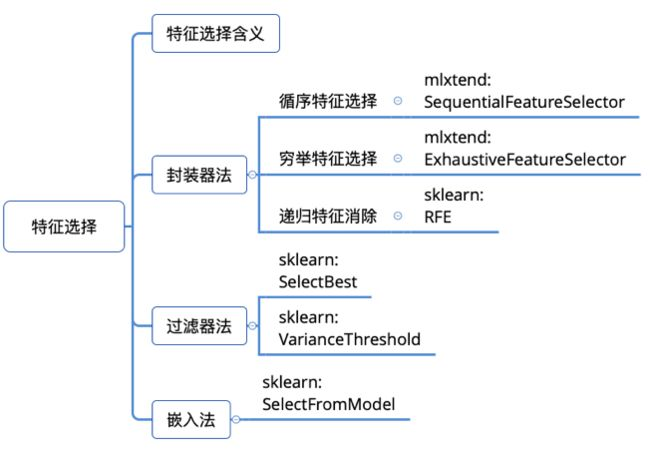
主要思想：包裹式（封装器法）从初始特征集合中不断的选择特征子集，训练学习器，根据学习器的性能来对子集进行评价，直到选择出最佳的子集。包裹式特征选择直接针对给定学习器进行优化

 

案例一、封装器法 

 

 

常用实现方法：循序特征选择。

• 循序向前特征选择：Sequential Forward Selection，SFS
• 循序向后特征选择：Sequential Backword Selection，SBS

SFS过程展示图：

 

 

 例子：

 

SequentialFeatureSelector(estimator, K_features=1, 
                          forvard=Truer,
                          floating=False, 
                          verhose=o , scoring=None,
                          cv=5, n_jobs=1, 
                          pre_dispatch-=2*n_jobs, 
                          clone_estimator=True)

 

加载数据集

#加载数据集
from mlxtend.feature_selection import SequentialFeatureSelector as SFS #SFS
from mlxtend.data import wine_data #dataset
from sklearn.neighbors import KNeighborsClassifier
from sklearn.model_selection import train_test_split
from sklearn.preprocessing import StandardScaler

X, y = wine_data()
X.shape  #(178, 13)

 

数据预处理

#数据预处理
X_train, X_test, y_train, y_test= train_test_split(X, y, stratify=y, test_size=0.3, random_state=1)
std = StandardScaler()
X_train_std = std.fit_transform(X_train)

 

循序向前特征选择

#循序向前特征选择
knn = KNeighborsClassifier(n_neighbors=3)

sfs = SFS(estimator=knn, k_features=4, forward=True, floating=False, verbose=2, scoring='accuracy', cv=0)
sfs.fit(X_train_std, y_train)  #xy不能是df

 

查看特征索引

#查看特征索引
sfs.subsets_

{1: {'feature_idx': (6,),
'cv_scores': array([0.86290323]),
'avg_score': 0.8629032258064516},
2: {'feature_idx': (6, 9),
'cv_scores': array([0.95967742]),
'avg_score': 0.9596774193548387},
3: {'feature_idx': (6, 9, 11),
'cv_scores': array([0.99193548]),
'avg_score': 0.9919354838709677},
4: {'feature_idx': (6, 8, 9, 11),
'cv_scores': array([0.98387097]),
'avg_score': 0.9838709677419355}}

可视化#1  Plotting the results

%matplotlib inline
from mlxtend.plotting import plot_sequential_feature_selection as plot_sfs
fig = plot_sfs(sfs.get_metric_dict(), kind='std_err') 

 

其中 sfs.get_metric_dict()的结果如下：

{1: {'feature_idx': (6,),
'cv_scores': array([0.86290323]),
'avg_score': 0.8629032258064516,
'ci_bound': nan,
'std_dev': 0.0,
'std_err': nan},
2: {'feature_idx': (6, 9),
'cv_scores': array([0.95967742]),
'avg_score': 0.9596774193548387,
'ci_bound': nan,
'std_dev': 0.0,
'std_err': nan},
3: {'feature_idx': (6, 9, 11),
'cv_scores': array([0.99193548]),
'avg_score': 0.9919354838709677,
'ci_bound': nan,
'std_dev': 0.0,
'std_err': nan},
4: {'feature_idx': (6, 8, 9, 11),
'cv_scores': array([0.98387097]),
'avg_score': 0.9838709677419355,
'ci_bound': nan,
'std_dev': 0.0,
'std_err': nan}}

可视化#2   Selecting the “best” feature combination in a k-range

knn = KNeighborsClassifier(n_neighbors=3)
sfs2 = SFS(estimator=knn, k_features=(3, 10),
                   forward=True, 
                   floating=True,   
                   verbose=0,
                   scoring='accuracy',
                   cv=5)
sfs2.fit(X_train_std, y_train)
fig = plot_sfs(sfs2.get_metric_dict(), kind='std_err')

 

 

 全部代码如下：

# -*- coding: utf-8 -*-
"""
Created on Tue Aug 11 10:12:48 2020

@author: Admin
"""

#加载数据集
from mlxtend.feature_selection import SequentialFeatureSelector as SFS #SFS
from mlxtend.data import wine_data #dataset
from sklearn.neighbors import KNeighborsClassifier
from sklearn.model_selection import train_test_split
from sklearn.preprocessing import StandardScaler

X, y = wine_data()
X.shape  #(178, 13)


#数据预处理
X_train, X_test, y_train, y_test= train_test_split(X, y, stratify=y, test_size=0.3, random_state=1)
std = StandardScaler()
X_train_std = std.fit_transform(X_train)


#循序向前特征选择
knn = KNeighborsClassifier(n_neighbors=3)

sfs = SFS(estimator=knn, k_features=4, forward=True, floating=False, verbose=2, scoring='accuracy', cv=0)
sfs.fit(X_train_std, y_train)

#查看特征索引
sfs.subsets_

#可视化#1  Plotting the results
%matplotlib inline
from mlxtend.plotting import plot_sequential_feature_selection as plot_sfs
fig = plot_sfs(sfs.get_metric_dict(), kind='std_err')  

#可视化#2   Selecting the “best” feature combination in a k-range
knn = KNeighborsClassifier(n_neighbors=3)
sfs2 = SFS(estimator=knn, k_features=(3, 10),
                   forward=True, 
                   floating=True,   
                   verbose=0,
                   scoring='accuracy',
                   cv=5)
sfs2.fit(X_train_std, y_train)
fig = plot_sfs(sfs2.get_metric_dict(), kind='std_err')

 

案例二、封装器之穷举特征选择

穷举特征选择（Exhaustive feature selection），即封装器中搜索算法是将所有特征组合都实现一遍，然后通过比较各种特征组合后的模型表现，从中选择出最佳的特征子集

导入相关库

#导入相关库
from mlxtend.feature_selection import ExhaustiveFeatureSelector as EFS
from sklearn.neighbors import KNeighborsClassifier
from sklearn.datasets import load_iris

 

加载数据集

#加载数据集
iris = load_iris()
X = iris.data
y = iris.target

 

穷举特征选择

#穷举特征选择
knn = KNeighborsClassifier(n_neighbors=3) # n_neighbors=3

efs = EFS(knn,
         min_features=1,
         max_features=4,
         scoring='accuracy',
         print_progress=True,
         cv=5)
efs = efs.fit(X, y)

 

查看最佳特征子集

#查看最佳特征子集
print('Best accuracy score: %.2f' % efs.best_score_)  #Best accuracy score: 0.97
print('Best subset(indices):', efs.best_idx_)         #Best subset(indices): (0, 2, 3)
print('Best subset (correponding names):', efs.best_feature_names_)  #没有这个函数 

 

度量标准

#度量标准
efs.get_metric_dict()


import pandas as pd

df = pd.DataFrame.from_dict(efs.get_metric_dict()).T
df.sort_values('avg_score', inplace=True, ascending=False)
df

 

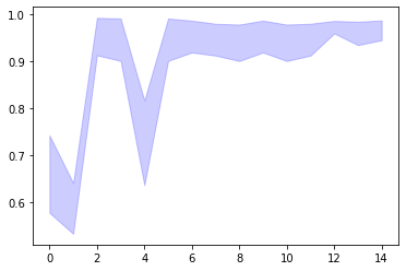
可视化

#可视化
import matplotlib.pyplot as plt

# 平均值
metric_dict = efs.get_metric_dict() 
k_feat = sorted(metric_dict.keys())
avg = [metric_dict[k]['avg_score'] for k in k_feat]

# 区域
fig = plt.figure()
upper, lower = [], []
for k in k_feat: #bound
    upper.append(metric_dict[k]['avg_score'] + metric_dict[k]['std_dev'])
    lower.append(metric_dict[k]['avg_score'] - metric_dict[k]['std_dev'])

plt.fill_between(k_feat, upper, lower, alpha=0.2, color='blue', lw=1)

# 折线图
plt.plot(k_feat, avg, color='blue', marker='o')

# x, y 轴标签
#无法运行
'''
plt.ylabel('Accuracy +/- Standard Deviation')
plt.xlabel('Number of Features')
feature_min = len(metric_dict[k_feat[0]]['feature_idx'])
feature_max = len(metric_dict[k_feat[-1]]['feature_idx'])
plt.xticks(k_feat, 
    [str(metric_dict[k]['feature_names']) for k in k_feat], 
    rotation=90)
plt.show()
'''

 

 全部代码如下：

# -*- coding: utf-8 -*-
"""
Created on Tue Aug 11 10:12:48 2020

@author: Admin
"""

#导入相关库
from mlxtend.feature_selection import ExhaustiveFeatureSelector as EFS
from sklearn.neighbors import KNeighborsClassifier
from sklearn.datasets import load_iris

#加载数据集
iris = load_iris()
X = iris.data
y = iris.target


#穷举特征选择
knn = KNeighborsClassifier(n_neighbors=3) # n_neighbors=3

efs = EFS(knn,
         min_features=1,
         max_features=4,
         scoring='accuracy',
         print_progress=True,
         cv=5)
efs = efs.fit(X, y)

#查看最佳特征子集
print('Best accuracy score: %.2f' % efs.best_score_)  #Best accuracy score: 0.97
print('Best subset(indices):', efs.best_idx_)         #Best subset(indices): (0, 2, 3)
print('Best subset (correponding names):', efs.best_feature_names_)  #没有这个函数 




#度量标准
efs.get_metric_dict()


import pandas as pd

df = pd.DataFrame.from_dict(efs.get_metric_dict()).T
df.sort_values('avg_score', inplace=True, ascending=False)
df

#可视化
import matplotlib.pyplot as plt

# 平均值
metric_dict = efs.get_metric_dict() 
k_feat = sorted(metric_dict.keys())
avg = [metric_dict[k]['avg_score'] for k in k_feat]

# 区域
fig = plt.figure()
upper, lower = [], []
for k in k_feat: #bound
    upper.append(metric_dict[k]['avg_score'] + metric_dict[k]['std_dev'])
    lower.append(metric_dict[k]['avg_score'] - metric_dict[k]['std_dev'])

plt.fill_between(k_feat, upper, lower, alpha=0.2, color='blue', lw=1)

# 折线图
plt.plot(k_feat, avg, color='blue', marker='o')

# x, y 轴标签
#无法运行
'''
plt.ylabel('Accuracy +/- Standard Deviation')
plt.xlabel('Number of Features')
feature_min = len(metric_dict[k_feat[0]]['feature_idx'])
feature_max = len(metric_dict[k_feat[-1]]['feature_idx'])
plt.xticks(k_feat, 
    [str(metric_dict[k]['feature_names']) for k in k_feat], 
    rotation=90)
plt.show()
'''

 案例三、过滤器法

 

 

例1

方差阈值（VarianceThreshold）是特征选择的一个简单方法，去掉那些方差没有达到阈值的特征。默认情况下，删除零方差的特征，例如那些只有一个值的样本。
假设我们有一个有布尔特征的数据集，然后我们想去掉那些超过80%的样本都是0（或者1）的特征。布尔特征是伯努利随机变量，方差为 p(1-p)。

使用方差选择法，先要计算各个特征的方差，然后根据阈值，选择方差大于阈值的特征。使用feature_selection库的VarianceThreshold类
方差选择法，返回值为特征选择后的数据 #参数threshold为方差的阈值

from sklearn.feature_selection import VarianceThreshold

X = [[0, 0, 1], [0, 1, 0], [1, 0, 0], [0, 1, 1], [0, 1, 0], [0, 1, 1]]
print(X)  #[[0, 0, 1], [0, 1, 0], [1, 0, 0], [0, 1, 1], [0, 1, 0], [0, 1, 1]]

sel = VarianceThreshold(threshold=(.8 * (1 - .8)))
sel.fit_transform(X)
'''
array([[0, 1],
       [1, 0],
       [0, 0],
       [1, 1],
       [1, 0],
       [1, 1]])
'''

例子2

X = [[0, 2, 0, 3], [0, 1, 4, 3], [0, 1, 1, 3]]
print(X)  #[[0, 2, 0, 3], [0, 1, 4, 3], [0, 1, 1, 3]]

seletor = VarianceThreshold()  #默认方法大于0
seletor.fit_transform(X)
'''
array([[2, 0],
       [1, 4],
       [1, 1]])
'''

 

案例四、嵌入法

对系数排序——即特征权重，然后依据某个阈值选择部分特征。
在训练模型的同时，得到了特征权重，并完成特征选择。像这样，将特征选择过程与模型训练融为一体，在模型训练过程中自动进行了特征选择，被称为“嵌入法” （Embedded）特征选择。

 在过滤式和包裹式特征选择方法中，特征选择过程与学习器训练过程有明显的分别。而嵌入式特征选择在学习器训练过程中自动地进行特征选择。嵌入式选择最常用的是L1正则化与L2正则化。在对线性回归模型加入两种正则化方法后，他们分别变成了岭回归与Lasso回归

例1

 

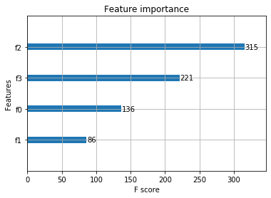
xgboost自带feature_importances_ 

 

#加载数据集
iris = load_iris()
X = iris.data
y = iris.target

#Xgboost特征重要性
from xgboost import XGBClassifier
model = XGBClassifier() # 分类
model.fit(X,y)
model.feature_importances_  # 特征重要性  array([0.01251974, 0.03348068, 0.59583396, 0.35816565], dtype=float32)

#可视化
%matplotlib inline
from xgboost import plot_importance
plot_importance(model)

 

 例2 

import matplotlib.pyplot as plt
import numpy as np

from sklearn.datasets import load_boston
from sklearn.feature_selection import SelectFromModel
from sklearn.linear_model import LassoCV

# Load the boston dataset.
X, y = load_boston(return_X_y=True)

# We use the base estimator LassoCV since the L1 norm promotes sparsity of features.
clf = LassoCV()

# Set a minimum threshold of 0.25
sfm = SelectFromModel(clf, threshold=0.25)
sfm.fit(X, y)
n_features = sfm.transform(X).shape[1]

# Reset the threshold till the number of features equals two.
# Note that the attribute can be set directly instead of repeatedly
# fitting the metatransformer.
while n_features > 2:
    sfm.threshold += 0.1
    X_transform = sfm.transform(X)
    n_features = X_transform.shape[1]
# Plot the selected two features from X.
plt.title(
"Features selected from Boston using SelectFromModel with " "threshold %0.3f." % sfm.threshold)
feature1 = X_transform[:, 0]
feature2 = X_transform[:, 1]
plt.plot(feature1, feature2, 'r.')
plt.xlabel("Feature number 1")
plt.ylabel("Feature number 2")
plt.ylim([np.min(feature2), np.max(feature2)])
plt.show()

 

 

 例3

from sklearn.feature_selection import SelectFromModel
from sklearn.linear_model import LogisticRegression
X = [[ 0.87, -1.34, 0.31 ],
    [-2.79, -0.02, -0.85 ],
    [-1.34, -0.48, -2.55 ],
    [ 1.92, 1.48, 0.65 ]]
y = [0, 1, 0, 1]
selector = SelectFromModel(estimator=LogisticRegression()).fit(X, y)

# The base estimator from which the transformer is built.
print(selector.estimator_.coef_)  #[[-0.32857694  0.83411609  0.46668853]]

# The threshold value used for feature selection.
print(selector.threshold_)  #0.5431271870420732

# Get a mask, or integer index, of the features selected
print(selector.get_support)

# Reduce X to the selected features.
selector.transform(X)

'''
array([[-1.34],
       [-0.02],
       [-0.48],
       [ 1.48]])
'''